Reverse a specified appraisal-smoothing model to estimate latent returns, with a 0.5% worked example and clear limits on volatility recovery and identification.
Return unsmoothing
Return unsmoothing is the inversion of a specified smoothing model to estimate the underlying returns behind a lagged, appraisal-based return series. Its practical purpose is to assess whether reported stability understates the risk an investor is taking. The recovered series is an estimate conditional on the model, not a set of verified transaction prices.
In commercial property, an appraisal may retain information from an earlier valuation because current comparable transactions are sparse. That can spread a market movement across reporting periods. Geltner’s 1991 analysis studies the resulting distortion of second moments. Clayton, Geltner and Hamilton (2001) find evidence of appraisal lag and that its extent varies with the information available to appraisers.
Remove the old information before rescaling
Consider a deliberately simple one-period partial-adjustment model:
rtobs=(1−θ)rt∗+θrt−1obs,0≤θ<1.
Here rtobs is the reported return, rt∗ is the unobserved current return and θ is the weight carried over from the previous reported return. All returns use the same reporting frequency and definition. This is a stipulated linear return model; it is not an accounting identity that every appraisal index must satisfy.
Given θ, its inverse is
rt∗=1−θrtobs−θrt−1obs.
Suppose the previous reported return was 2.0%, the current reported return is 1.4%, and the assumed smoothing weight is 0.60. Then
rt∗=0.400.014−0.60(0.020)=0.005=0.5%.
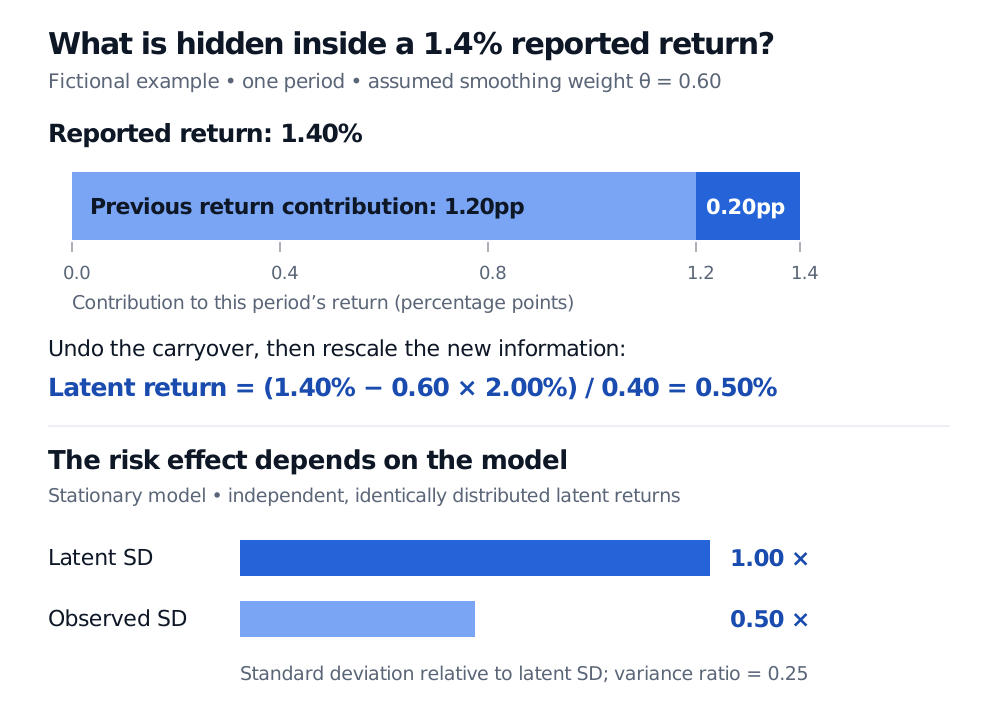
The reported 1.4% comprises 1.2 percentage points of carryover and 0.2 percentage points of current information. Dividing that remaining 0.2 by the current-information weight of 0.40 gives 0.5%. An unsmoothed return can therefore be smaller in a particular period even when the reconstructed series is more volatile overall.
Fictional partial-adjustment example with smoothing weight 0.60: reported return 1.40% contains 1.20 percentage points from the previous reported return and 0.20 from the current latent return. Inversion gives latent return 0.50%. Under stationary iid latent returns, observed standard deviation is half latent standard deviation and observed variance is one quarter.
The first panel decomposes one fictional return; the second shows a population risk identity under additional stationary iid assumptions. Neither panel estimates a real asset’s smoothing weight.
When the volatility correction has a clean answer
Assume now that θ is constant and that latent returns are independent and identically distributed with finite variance σ∗2. Take the reported process in its stationary distribution, so initialization effects have disappeared. Current latent returns are then independent of past reported returns. Taking variances gives
σobs2=(1−θ)2σ∗2+θ2σobs2,σ∗2σobs2=1+θ1−θ.
For θ=0.60, observed variance is 0.25 times latent variance, and observed volatility, measured as standard deviation, is 0.50 times latent volatility. Under these same assumptions, the lag-one autocorrelation of reported returns equals θ, hence 0.60.
These are population identities under the stated model. Finite samples need not match them exactly. Autocorrelated latent returns, changing appraisal weights or additional measurement noise change the calculation.
Serial dependence does not identify its cause
Setting θ equal to a sample autocorrelation assumes that the observed persistence comes entirely from this smoothing mechanism. Genuine return predictability, overlapping return windows and omitted economic dynamics can also produce persistence. Removing all of it may remove genuine structure. Geltner’s 1993 approach explicitly allows underlying market returns to remain correlated; the simple iid illustration above is a narrower model.
The inverse also magnifies errors. Holding the previous observation and θ fixed, a 0.1-percentage-point error in the current reported return becomes a 0.25-percentage-point error in the recovered return at θ=0.60. At θ=0.90, it becomes 1 percentage point. The multiplier is 1/(1−θ). Errors in the estimated weight create additional uncertainty; near one, the inverse becomes particularly sensitive.
An implausible reconstructed simple return below −100% is a reason to investigate the model, data and return convention. It is not evidence that an unlevered asset actually lost more than its entire value. Unsmoothing also creates no trading liquidity: an estimated latent return says nothing by itself about an executable sale price or how quickly the asset can be sold.
For portfolio work, examine sensitivity to plausible weights and valuation mechanisms before using the recovered series in a portfolio volatility estimate. Frei (2024) warns that unsmoothing heavily smoothed series can overstate volatility and need not fully recover cross-asset correlations. A more jagged series alone does not establish a better risk model.