A fixed recurrent reservoir turns input history into features; a trained readout makes predictions. See a pulse-memory example and the limits of spectral-radius rules.
Reservoir computing and echo-state network
Reservoir computing turns a sequence into evolving features using a dynamical system, then learns a readout from those features. An echo-state network (ESN) is a recurrent-neural-network implementation: in its classical form, input and recurrent weights are chosen first and held fixed while the output weights are fitted. For a quant modelling a financial time series, this replaces training the recurrent dynamics with a simpler supervised output fit. It does not establish that the resulting features contain a useful forecasting signal. Jaeger's adaptive ESN paper develops this separation and an online readout update.
What stays fixed, and what learns?
Consider an ESN without output feedback or leaky integration:
ht=tanh(Wht−1+Uxt+b),zt+1=c+vTht.
Here xt is the current input vector, ht is the reservoir state, W supplies recurrent connections, U maps inputs into the reservoir, and b is a reservoir bias. The hyperbolic tangent acts component by component. In this setup, W, U and b remain fixed; the readout coefficients v and intercept c learn the mapping to the target zt+1.
This is still a recurrent neural network: the state changes every time an input arrives. Fixed reservoir weights do not mean a fixed forecast. The same reservoir can also support different readouts for different targets. Unlike full recurrent training, fitting this readout does not require backpropagating a loss through the state recursion.
A pulse leaves a trace
Take a deterministic, one-unit reservoir with dimensionless inputs:
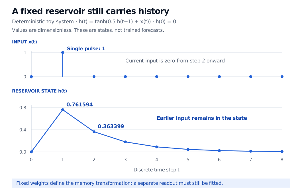
At the second step, the current input is zero, but the state is positive because it carries the earlier pulse. Starting at zero and feeding two zeros instead would give a zero state. Thus two histories with the same current input can produce different reservoir features.
A deterministic one-unit reservoir receives an input of 1 at step 1 and 0 afterward. Its state rises from 0 to 0.761594, falls to 0.363399 at step 2, and decays toward zero through step 8. The state is a feature, not a trained forecast.
Figure: A fixed nonlinear recurrence preserves a fading trace of a past input. Dots are discrete updates; connecting lines guide the eye. No readout is fitted in this toy example.
The values above are reservoir activations. A volatility or return forecast would require a separately fitted readout and appropriately defined training targets; neither value is itself a market prediction.
What the “echo” property promises
The echo-state property concerns forgetting initial conditions under the specified driving inputs: the reservoir response becomes determined by input history rather than an arbitrary starting state. Its scope includes the admissible inputs and states. Input-dependent formulations make this dependence explicit; it is not solely a property of one weight-matrix number. Manjunath and Jaeger explain that distinction.
For the displayed tanh update with no output feedback, a useful sufficient condition is
∥W∥2<1,
where this induced Euclidean operator norm is the largest singular value. Since componentwise tanh is 1-Lipschitz, two trajectories driven by the same inputs obey
∥ht−ht∥2≤∥W∥2t∥h0−h0∥2.
On the invariant state cube, this contraction removes dependence on the initial state. Our scalar example has contraction factor at most 0.5. Jaeger's corrected report, Proposition 3(a), gives this sufficient condition; its 2010 erratum corrects a separate state-contraction definition in the original report.
The spectral radius, the largest absolute eigenvalue, is different from that norm. Scaling it below one is a common ESN heuristic, not a universal necessary-and-sufficient test across activations, inputs and architectures. Input forcing can change the relevant dynamics. See Lukoševičius, §3.2.4.
Fitting the output still needs discipline
A simple ridge-regression readout minimises
t∈T∑(zt+1−c−vTht)2+λ∥v∥22,λ≥0.
Here T contains training times and the intercept is unpenalised. Regularisation controls the readout, not the reservoir's echo-state property. Reservoir size, input scaling and memory dynamics still need validation. For long streams, an initial washout can exclude states dominated by initialization; its length depends on the dynamics, and discarding a transient is not proof of the echo-state property. These training choices are discussed in Lukoševičius, §§3–4.
For a financial forecast, align each state with information available at its prediction time to avoid look-ahead bias. Fit scaling and readout parameters on training data, select settings on later validation data, and assess the selected model on an untouched later period. Continuing a state into validation is coherent for one continuous stream when only past inputs drive it; independent sequences need an explicit reset policy. Cheap readout fitting does not remove these timing decisions.