How projection pursuit regression learns smooth responses to combinations of predictors, with a checked geometric example and guidance on fitting and identification.
Projection pursuit regression
Projection pursuit regression (PPR) predicts a response by adding smooth functions of learned linear combinations of the predictors. A quant can use it to model a nonlinear response to a combination of financial signals, rather than requiring a separate curve for each signal. Its directions are learned using the response, so they describe predictive associations rather than automatically identifying economic factors or causal effects.
Additive after projection
For a numeric response, write the fitted conditional-mean model as
f^(x)=β0+m=1∑Mgm(amTx),∥am∥2=1.
Each direction am combines the inputs into one scalar. Its smooth gm then maps that scalar into a response contribution. Any separate amplitude coefficient can be absorbed into gm in this notation. Friedman and Stuetzle introduced the method as an iterative sum of smooths of linear combinations. Their original paper develops the search and smoothing steps; the author preprint makes these explicit in §§2–4.
A basic generalised additive model adds curves of the original coordinates. PPR is additive in its learned projections instead. Consequently, it can contain interactions between the original predictors even when there is only one term.
Here, a ridge function means a function x↦g(aTx): it is constant along directions perpendicular to a. This geometric use of “ridge” does not mean the coefficient penalty in ridge regression.
A prediction you can inspect
Consider two dimensionless inputs and a stipulated one-term predictor with zero intercept:
a=(0.6,0.8)T,x=(3,4)T,g(u)=u2.
The direction has unit length because 0.62+0.82=1. Therefore
u=aTx=0.6(3)+0.8(4)=5,f^(x)=g(5)=25.
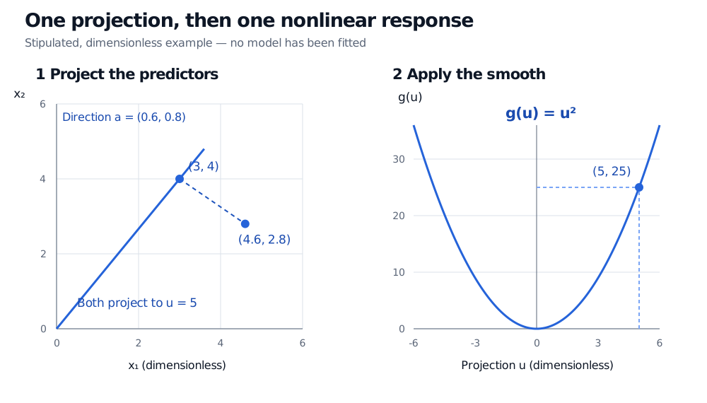
These are supplied parameters, not estimates recovered from training data; the output is dimensionless, not a forecast return. The point (4.6,2.8) has the same projection, hence the same prediction. Its displacement from (3,4) is perpendicular to a.
Two input points, (3,4) and (4.6,2.8), both project to 5 along the unit direction (0.6,0.8). The quadratic smooth maps projection 5 to prediction 25.
Figure: Original dimensionless illustration of a stipulated predictor. The dashed segment joins equal-projection points; the right panel applies the nonlinear response curve.
Expanding this particular predictor reveals what coordinatewise additivity would miss:
(0.6x1+0.8x2)2=0.36x12+0.96x1x2+0.64x22.
The cross-product is an interaction. Also, the direction entries are not constant marginal effects: the derivatives are 1.2u and 1.6u, giving 6 and 8 at the example point. A loading describes how an input moves the projection; the slope of the smooth determines how that movement changes the prediction.
What fitting has to learn
The original algorithm searches for a direction whose smoothed projection explains the current residuals, adds that term, and continues. Backfitting can readjust earlier terms. Numerical searches can reach local optima; one-dimensional smoothing simplifies each component without making the whole learning problem trivial. The current R ppr documentation illustrates an implementation that adds candidate ridge terms, then removes terms, with controls for smoothing and refitting.
PPR differs from principal component analysis: PCA chooses directions to retain predictor variance without using the response. PPR chooses directions to fit the response. PPR directions need not be mutually orthogonal, and a high-variance input direction need not be predictively useful.
There are representation ambiguities. Multiplying a direction by a nonzero constant can be offset by rescaling the smooth's argument; reversing its sign can be offset by reflecting the smooth. Unit-length directions remove the scale ambiguity. A reporting sign convention, such as making the first nonzero loading positive, resolves the sign choice. Centre each smooth over the training observations and transfer its constant into the intercept. These conventions make plots comparable, but do not guarantee a unique decomposition when several terms can represent the same surface. The worked example uses the uncentred curve for transparent arithmetic; centring would redistribute its constant without changing predictions.
Using it with financial observations
Control the number of terms and smoothness using cross-validation; a lower training error alone does not establish better prediction. Fit preprocessing, directions and smooths within each training fold. Apply the resulting transformations to validation observations, and keep the final test period out of model selection. Learning even a scaling transformation from the full sample leaks information, as the scikit-learn leakage guidance explains.
For a forecasting application, validation must also respect the time when predictors and target labels become available. A smooth learned in one market regime may not transfer to another. Inspect each curve where projected training observations actually lie: the formula's ability to return a number outside that range does not validate extrapolation.