NGBoost predicts conditional distributions with natural-gradient boosting. See how a Normal mean and scale update, why trees and line search matter, and how to assess forecast uncertainty.
NGBoost
NGBoost (Natural Gradient Boosting) is a supervised learning method that uses boosting to estimate a conditional probability distribution for an outcome. A quant model can therefore predict both the location and spread of a future return, rather than attaching the same uncertainty band to every point forecast. The distribution remains a modelling assumption: fitting its parameters does not establish that its tail probabilities are reliable.
Different features can imply different means and standard deviations. The official Python library distinguishes predict(), which returns point predictions, from pred_dist(), which returns conditional distribution objects. Its Normal model reports loc and scale, meaning the mean and standard deviation. Official usage guide.
Why the natural gradient matters
Ordinary gradient boosting fits successive learners to loss-based corrections. NGBoost extends this to several distribution parameters, using a proper scoring rule to judge each predicted distribution against the observed outcome.
A raw gradient depends on the coordinates used for those parameters. Changing a mean by one unit and changing a log standard deviation by one unit have different effects on the distribution. NGBoost rescales the gradient using a local metric induced by the scoring rule. For negative log-likelihood, that metric is the Fisher information matrix. For another score, the corresponding metric can differ. Duan et al., §§3.1–3.2.
The resulting natural-gradient direction describes a local change in the distribution. This geometric property does not mean that arbitrary finite steps, fitted trees or complete training runs become identical under every reparameterisation.
Isolating one mean-and-scale correction
Consider one synthetic observation, y=1, in dimensionless toy units. Start with μ=0 and σ=2, and write s=logσ. The negative log-likelihood is
L(μ,s;y)=21log(2π)+s+2e2s(y−μ)2.
Its gradient and Fisher information, in the coordinate order (μ,s), are
∇L=((μ−y)/σ21−(y−μ)2/σ2),I(μ,s)=(1/σ2002).
The Fisher matrix averages score outer products over possible outcomes under the current model. It is not the outer product of the gradient at this single observed outcome. These formulas match the library's Normal log-score implementation.
At the stated starting values,
∇L=(−.25.75),I−1∇L=(−1.375).
Take a standalone natural-gradient descent step of size η=0.1:
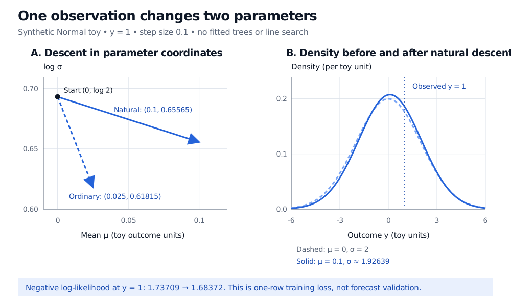
The mean moves toward the observation, while the distribution narrows because the observation is relatively close to the initial mean. Using the ordinary gradient with the same step size would instead move the mean to 0.025 and subtract 0.075 from the log standard deviation. Equal numerical step sizes therefore produce different balances between the two corrections.
Synthetic Normal toy with observation 1. A step of 0.1 moves mean and log standard deviation from (0, 0.69315) to (0.1, 0.65565) using the natural gradient, versus (0.025, 0.61815) using the ordinary gradient. The natural step gives standard deviation 1.92639 and reduces one-row negative log-likelihood from 1.73709 to 1.68372.
Original standalone natural-gradient illustration. The left panel uses zoomed parameter axes; the right shows the initial and updated densities. Trees and stage line search are omitted.
The natural step lowers this observation's negative log-likelihood from about 1.73709 to 1.68372. That is a calculation about one training observation; it supplies no evidence about future forecast quality.
Where the trees enter
The toy above omits the machinery that makes NGBoost a prediction model. In a full stage, the algorithm computes natural gradients for training rows, fits base learners to their components, and chooses a shared stage scaling by line search. It then applies the scaled learner outputs with shrinkage. New inputs receive corrections through those fitted functions of the features. The learners approximate the gradient field; they need not reproduce each row's gradient exactly. Duan et al., §3.4 and Algorithm 1; current implementation.
For the sequential-fitting background, Boosting: AdaBoost and Gradient Boosting develops residual fitting and shrinkage. Its full teaching requires membership; a public preview is available.
A distribution still needs validation
An estimated conditional spread describes outcome uncertainty within the fitted distribution family. It is not automatically a Bayesian posterior over models, nor a separate allowance for uncertainty about the estimated parameters. A Normal forecast can miss skewness and heavy tails even when its mean and scale vary with features.
Assess distributional forecasts on held-out outcomes: compare a proper score such as negative log-likelihood, check prediction-interval calibration, and inspect performance across relevant market regimes. Interval coverage alone can hide excessively wide forecasts, so examine sharpness alongside coverage. These checks answer different questions from point-prediction error.
The official tuning guide supports validation-loss tracking, staged prediction and early stopping. In financial data, the split must also respect information availability and overlapping outcome windows. Finance-aware validation works through purging and embargoes; its full lesson requires membership, with a public preview. Good optimisation cannot repair leakage or make a misspecified distribution valid.