Neural tangent kernel: Definition & Examples

The neural tangent kernel (NTK) measures how similarly two inputs respond to small changes in a model's parameters. For a quant training a neural network on financial features, it offers a way to study how correcting one observation changes predictions on others—and whether training is behaving much like a fixed kernel method.

For a differentiable model with scalar output

f_\theta(x)

and parameter vector

\theta\in\mathbb{R}^P

, its finite NTK is

K_\theta(x,x')=\nabla_\theta f_\theta(x)^\top\nabla_\theta f_\theta(x').

The features here are parameter derivatives, not the raw inputs. Two observations can have a large kernel value because the same parameter changes move their predictions together. This is a local, parameterization-dependent relationship: changing parameter scales can change the NTK even if the model can represent the same functions. The finite kernel generally changes during nonlinear training. This definition and its training interpretation come from Jacot, Gabriel and Hongler, §4.

From weight changes to prediction changes

On $n$ training observations, collect predictions in $\mathbf f_\theta$ and let the $n\times P$ Jacobian $J_\theta$ have row $i$ equal to $\nabla_\theta f_\theta(x_i)^\top$ . The training Gram matrix is

\mathbf K_\theta=J_\theta J_\theta^\top.

It is positive semidefinite: for any vector

\mathbf c

\mathbf c^\top\mathbf K_\theta\mathbf c=\lVert J_\theta^\top\mathbf c\rVert^2\ge0

. It need not be invertible.

Use the half sum of squared errors, with no division by the sample count:

L(\theta)=\frac12\sum_{i=1}^{n}\bigl(f_\theta(x_i)-y_i\bigr)^2.

Ordinary Euclidean gradient descent gives $\Delta\theta=-\eta J_\theta^\top(\mathbf f_\theta-\mathbf y)$ . A first-order expansion then gives

\Delta\mathbf f\approx-\eta\mathbf K_\theta(\mathbf f_\theta-\mathbf y).

For a nonlinear model, a finite step has an approximation error. Under continuous-time gradient flow the chain rule instead gives the exact instantaneous identity $\dot{\mathbf f}_t=-\mathbf K_{\theta(t)}(\mathbf f_t-\mathbf y)$ . Neither statement freezes the kernel. Averaging the loss would introduce a factor $1/n$ ; adaptive optimizers require a different update analysis.

An exact two-observation example

Take the affine model $f_\theta(x)=ax+b$ , with $\theta=(a,b)$ , so $\nabla_\theta f_\theta(x)=(x,1)^\top$ and $K(x,x')=xx'+1$ . This is a deliberately small linear-in-parameters model, not an approximation to a hidden-layer network.

At inputs $1$ and $2$ ,

\mathbf K=\begin{pmatrix}2&3\\3&5\end{pmatrix}.

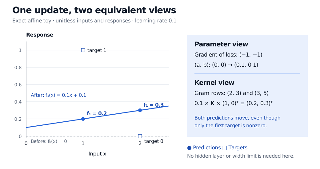
Start from $a=b=0$ , with targets $\mathbf y=(1,0)^\top$ and step size $\eta=0.1$ . Direct differentiation gives $\nabla L=(-1,-1)^\top$ , hence the new parameters are $(0.1,0.1)$ . Evaluating the updated model gives predictions $(0.2,0.3)^\top$ .

The kernel calculation agrees exactly:

\mathbf f_1=\mathbf f_0+0.1\mathbf K\mathbf y =\begin{pmatrix}0.2\\0.3\end{pmatrix}.

Exact affine toy with unitless inputs 1 and 2 and targets 1 and 0. Starting from zero predictions, a parameter update to a=b=0.1 gives predictions 0.2 and 0.3, matching the kernel calculation.

Original deterministic example. The blue line is the updated affine model; squares mark targets and circles mark predictions. The second prediction rises because its derivative features overlap those of the first observation.

The second observation initially has zero error, yet its prediction moves away from its target. The update follows the gradient of the aggregate loss; it does not promise to improve every observation separately. Here the derivative features stay fixed because the model is affine in its parameters, making the kernel step exact at any parameter value.

When does a neural network have a fixed kernel?

Jacot and coauthors prove a deterministic, fixed-kernel limit for suitably scaled fully connected networks as hidden-layer widths grow. Their training theorem assumes a Lipschitz, twice differentiable activation with bounded second derivative and bounded integrated training direction over the time interval. The width limit, parameter scaling and regularity assumptions matter; the finite definition alone supplies no such guarantee. See their model and Theorem 2.

Lazy training describes training that remains close to the model's linearization around initialization. Chizat, Oyallon and Bach, §§1.1–1.2 show that scaling is central, and that this behavior is not exclusive to large neural networks. A fixed tangent feature map can still yield nonlinear functions of the input. What it restricts is the evolution of the representation during training.

For financial prediction, a frozen-NTK model can therefore serve as a comparison against a network whose derivative features evolve. Agreement helps diagnose the training regime; disagreement can reveal where the local approximation breaks down. Neither finding establishes out-of-sample forecasting value, protection against changing markets, or calibrated predictive uncertainty. An NTK describes training sensitivity, not automatically a probabilistic forecast distribution.

For the underlying feature-map and Gram-matrix algebra, see The Kernel Trick: Feature Maps and Properties of Kernels (public preview; full lesson requires membership).

Sources

Jacot, Gabriel and Hongler (2018), Neural Tangent Kernel: Convergence and Generalization in Neural Networks: §2 parameter scaling; §4 finite NTK and limiting theorems; §5 least-squares dynamics. The linked author manuscript is the revised 2020 version.
Chizat, Oyallon and Bach (2019), On Lazy Training in Differentiable Programming: §§1.1–1.2 linearization and scaling. The linked author manuscript is the revised 2020 version.

From weight changes to prediction changes

An exact two-observation example

When does a neural network have a fixed kernel?

Sources

Related terms

Neural network

Positive semidefinite matrix