Read neural scaling laws as conditional empirical loss relationships, distinguish excess from total loss, and separate training compute allocation from inference cost.
Neural scaling laws
Neural scaling laws are empirical relationships describing how a neural network's loss changes as model size, training data or training compute increases within a specified experimental regime. For a quant team, they can inform the next training experiment and its budget; they do not establish the accuracy or profitability of a financial application.
First ask what is being scaled
The three quantities answer different questions:
Quantity
What it measures
What to keep explicit
Parameters, N
The size of the fitted model
Which parameters count, architecture and training procedure
Data, D
Dataset size or training tokens processed, as defined in the study
Unique observations versus repeated exposure, tokenisation and data quality
Training compute, C
Arithmetic used during training, usually measured in FLOPs
How compute is divided between model size and training exposure
A model-size curve asks what happens when N changes under its stated data and training conditions. A sample-size learning curve varies data. A compute-optimal frontier instead selects the best allocation of resources at each compute budget. Their slopes need not agree.
Kaplan et al. (2020) reported power-law relationships for language-model cross-entropy, distinguishing parameter-, data- and compute-limited regimes. Their simple one-factor fits require the other factors not to be bottlenecks. “Law” here names a measured regularity, rather than a theorem applying to every neural network.
Half of which loss?
Consider a hypothetical stipulated relationship, with N measured numerically in millions of parameters and loss in arbitrary units:
L(N)=1+2N−1/2.
The floor of 1, coefficient 2 and exponent 1/2 are teaching choices, not empirical estimates. Changing the units of N changes the coefficient needed to describe the same curve.
Model size
Total loss
Excess above the stipulated floor
N=100
1+2/10=1.2
0.2
N=400
1+2/20=1.1
0.1
Four times as many parameters halves the excess because
L(100)−1L(400)−1=0.20.1=21.
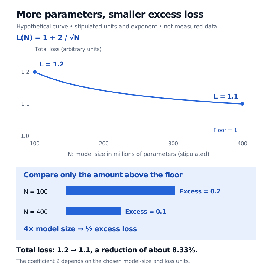
Total loss falls by 0.1, or about 8.33% of its initial 1.2. It does not halve. More generally, for a positive excess L(N)−L∞=AN−α, multiplying N by k multiplies the excess by k−α. A straight line on log–log axes describes that excess; adding a floor changes the shape of the total-loss curve.
Hypothetical stipulated curve: N rises from 100 to 400 million parameters, total loss falls from 1.2 to 1.1 arbitrary units, and excess above floor 1 falls from 0.2 to 0.1.
Original hypothetical illustration. Quadrupling model size halves excess loss; total loss falls about 8.33%. The displayed range and all coefficients are stipulated, with no measured data or fitted exponent.
with coefficients estimated from training runs. In this compute approximation, model size is counted in individual parameters and data in training tokens, rather than the toy's millions-of-parameters units. For the dense-transformer approximation C≈6ND, increasing N at fixed C leaves fewer training tokens. The allocation problem is to minimise the fitted loss subject to that compute constraint. The constrained optimisation lesson explains the mathematical machinery (membership; public preview available). A fitted loss surface does not make neural-network training itself a convex problem.
Kaplan's compute allocation favoured faster growth in parameters than data. Hoffmann's estimates favoured roughly equal growth. Hoffmann varied training horizons with matching learning-rate schedules and used a different model-size range; the fitting regimes differ. These are historical empirical estimates, not competing universal constants. In Chinchilla's analysis, training exposure remained below one dataset epoch.
The training constraint also omits deployment usage. An inference budget concerns serving requests after training: latency, memory, request volume and generation length matter. Minimising pretraining loss at fixed training FLOPs does not by itself minimise lifetime cost.
Use the fit as a research hypothesis
A scaling experiment needs comparable objectives, data definitions and evaluation procedures. Fit across several sizes, inspect residuals and uncertainty, and test predictions on additional runs before committing to a larger scale. A fitted floor is an estimate under that model, not a discovered universal limit. Kaplan explicitly identified eventual breakdown of extrapolated trends; Chinchilla also discussed frontier curvature and extrapolation uncertainty.
For financial text, lower token-prediction cross-entropy does not certify a return forecast, a correct extracted earnings figure or a useful risk decision. Those require task-specific evaluation. Repeated documents and overlapping market labels also make raw counts a poor substitute for independent evidence.
Use the time-ordered validation lesson to separate fitting, model selection and final assessment while respecting information availability (membership; public preview available). If evaluation results guide the choice of scale, they are development evidence. Preserve a final test set for the frozen procedure.
Sources
Kaplan, J. et al. (2020), Scaling Laws for Neural Language Models, §§1.2, 5–6, especially §6.3: conditional power-law regimes, training compute allocation and eventual extrapolation breakdown.
Hoffmann, J. et al. (2022), Training Compute-Optimal Large Language Models, §§2–3 and 5, Appendices D.2 and E: training-horizon differences, joint loss fitting, allocation estimates and limits.