A neural oblivious decision ensemble (NODE) is the tabular deep-learning architecture introduced by Sergei Popov, Stanislav Morozov and Artem Babenko: it combines differentiable oblivious decision trees and trains them jointly through backpropagation. For a quant working with rows of asset characteristics, it offers a way to learn tree-like interactions together with intermediate representations. NODE names a particular architecture, rather than every neural model with soft tree routing. Original paper, §3.
What “oblivious” constrains
In an ordinary decision tree, two nodes at the same depth can use different tests. An oblivious tree shares the splitting feature and threshold across every node at a given depth. Different depths can use different tests. A depth- binary tree therefore has shared tests and a response table with entries. The constraint concerns routing, not identical leaf predictions. Paper, §2.
The Decision Trees: Splitting Criteria and Pruning lesson develops conventional recursive splitting and leaf predictions, which provide the comparison here. Its preview is public; the full lesson requires membership.
From a table lookup to weighted routing
The differentiable construction uses learned feature-selection weights to form a feature combination at each depth. A learned threshold and scale then determine soft branch weights. Entmax can give some features exactly zero selection weight; its binary counterpart is called entmoid in the authors' code. The original experiments use entmax with . A soft selection need not choose just one feature. Paper, §§3.1 and 4.1, authors' entmax/entmoid implementation.
For each leaf, multiply the branch weights along its path; the tree output is the weighted sum of its response values. The authors' ODST forward method implements feature selection, scaled threshold comparisons, path-weight products and response aggregation. Those operations allow gradients of the loss function to flow into routing parameters and leaf responses.
Consider a synthetic depth-two tree. Label a branch by bit 0 or 1. Number leaves from zero, with the first bit as the most significant bit: . The ordered paths 00, 01, 10 and 11 have stipulated responses 0, 1, 3 and 4. Hard routing with bits selects index 2, so the output is 3. This indexing convention is explicit; implementations can store the same table in another order.
Now stipulate soft branch-1 weights and . Branch-0 weights are their complements. These numbers illustrate aggregation; they are not outputs from a fitted entmoid gate.
| Path | Leaf response | Path weight | Weighted contribution |
|---|---|---|---|
| 00 | 0 | 0 | |
| 01 | 1 | 0.05 | |
| 10 | 3 | 1.80 | |
| 11 | 4 | 0.80 |
The weights sum to 1, and the output is
It lies between the smallest and largest responses because the weights are nonnegative and sum to one. These are routing weights, not probabilities of future market outcomes. The product rule is a deterministic part of the architecture; it does not assert that economic variables are statistically independent.
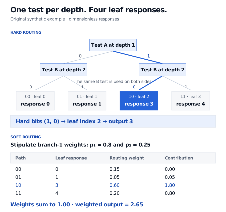
Original synthetic routing example. Tests A and B may differ; each is shared within its depth. The hard and soft evaluations use the same response table. All values are dimensionless; no model has been fitted.
An ensemble inside a deeper model
The paper's multilayer design passes original inputs and earlier tree outputs into later NODE layers, then averages prediction coordinates across trees. Parameters are trained jointly; this differs from adding residual-fitting trees sequentially in gradient boosting. Paper, §§3.2–3.3.
Tree depth and layer count describe different dimensions of complexity. Increasing depth expands each tree's response table exponentially. Adding layers allows later tests to act on learned intermediate outputs. Neither operation guarantees better forecasts.
For financial research, compare NODE with appropriate simpler baselines under the same time-ordered evaluation. Fit preprocessing and any data-aware initialisation using eligible training observations; future rows must not influence a historical fit. Select hyperparameters using development data and preserve a later test period. The paper's tabular benchmarks do not establish trading profitability or superiority on a particular financial dataset.
Finally, a large feature-selection weight describes an internal routing choice. It is not a causal effect or a complete measure of feature importance: downstream responses, repeated uses and correlated inputs also affect predictions. Differentiability makes training possible; it does not by itself prevent overfitting.
Sources
- Popov, Morozov and Babenko, Neural Oblivious Decision Ensembles for Deep Learning on Tabular Data, arXiv:1909.06312v2 (2019), §§2–3 and §4.1. Defines the oblivious constraint, differentiable routing, dense layer connections and experimental setup.
- Authors' supplementary implementation: ODST parameterisation and forward evaluation and entmax/entmoid functions. The worked routing values and figure are original synthetic examples.