A neural Hawkes process is a model for typed event arrivals whose conditional intensities are generated by a continuous-time recurrent neural network. For a quant modelling order arrivals, it offers a way to forecast which event comes next and when, using the timing and sequence of earlier events rather than just their total count.
Memory changes while the clock runs
The original Mei–Eisner model uses a continuous-time long short-term memory network: events update its memory, and memory cells evolve toward learned targets between arrivals. Thus the intensity can change even when no new event occurs. Unlike an additive, positive-kernel Hawkes process, it can represent order-dependent excitation and inhibition. These are predictive dependencies, not proof that one event causes another. Mei and Eisner, §§1 and 3.2.2.
The rate for event type is read from the hidden vector :
This scaled softplus keeps intensity positive even with signed readout weights. The scalar preactivation is not itself a probability or one bounded hidden-state component. A negative contribution may lower the rate without making the rate negative. Mei and Eisner, equations (3)–(4).
For the underlying memory gates, Gated Memory: LSTMs and GRUs explains cell state, forgetting and input gates. Its public page is a preview; the full lesson requires membership. That lesson covers ordinary discrete-step cells; the between-event evolution is the additional mechanism here.
A rate of two is not a probability of two
An intensity has units of events per unit time. For a sufficiently short interval, rate times interval length approximates an arrival probability conditional on the history immediately before it. A finite waiting probability instead needs integrated intensity. Rasmussen, §2.3.
Consider a stipulated scalar readout, with softplus scale one and time measured in one fixed unit. Choose the preactivation
Then : the intensity is 2 events per time unit. This calculation specifies only a readout value, not a trained continuous-time LSTM.
Now additionally hold that intensity constant for the next 0.5 time units. Its integrated hazard is
The conditional probability that no next event arrives in that window is , or 36.79%. The probability of at least one arrival is therefore 63.21%. The number one here is an accumulated hazard, not a 100% event probability.
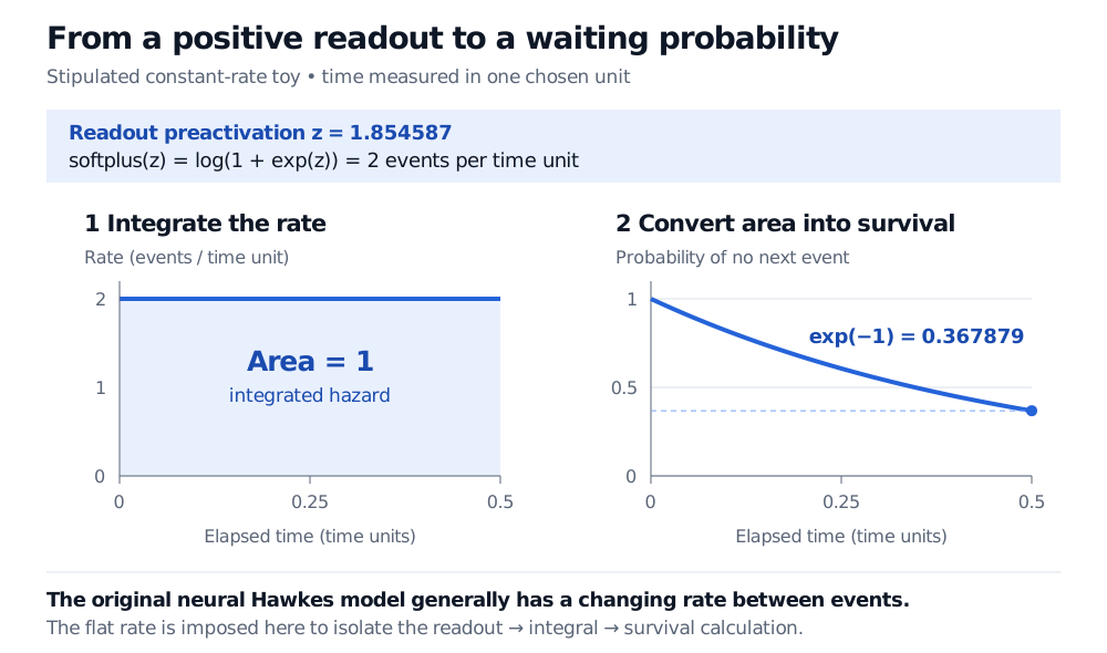
Original calculation diagram. The rate is held constant by assumption; this is a readout and survival illustration, not a fitted neural Hawkes model or market data.
For multiple event types, let be the forecast origin and the observed event history through that time. Evaluate each future intensity along the continuation in which no further event has yet occurred. The next-event survival function is
That conditioning matters: once an event happens, it updates the state. In the original model, even the no-event continuation generally has time-varying intensity. Freezing today's rate would replace that continuation with a different approximation. Rasmussen, §§2.3–2.4.
What the training objective asks
On an observation window , the event-stream log-likelihood combines the intensities assigned to observed types and times with an integral penalty:
Use the history just before each event for its intensity. The integral scores the waiting periods too; rewarding observed arrivals alone would favour inflated rates. Rasmussen, §3.1.
For financial use, define what counts as an event, its timestamp and its type before fitting. Assess forecasts on later periods with the same observation convention. Missing events or a changed recording process change the history the model sees; better timing prediction does not by itself establish profitable execution or an intervention effect.
Sources
- Hongyuan Mei and Jason Eisner, The Neural Hawkes Process: A Neurally Self-Modulating Multivariate Point Process (NeurIPS 2017), §§1, 3.2.1–3.2.2 and 4: continuous-time memory, positive readout and event-stream inference.
- Jakob Gulddahl Rasmussen, Lecture Notes: Temporal Point Processes and the Conditional Intensity Function (2018), §§2.3–2.4 and 3.1: conditional intensity, next-event distribution, marks and likelihood.