Understand backcast subtraction and additive forecasts in N-BEATS, then see how N-HiTS uses input pooling and hierarchical output interpolation for multi-step forecasting.
N-BEATS and N-HiTS
N-BEATS and N-HiTS are related neural architectures for multi-step forecasting. They build a future path by adding block contributions. For a quant forecasting a sequence of funding needs or trading volumes, they offer an alternative to recursively feeding each prediction back into a one-step model. Neither architecture establishes that the chosen financial target is predictable.
N-BEATS means Neural Basis Expansion Analysis for Time Series. N-HiTS means Neural Hierarchical Interpolation for Time Series Forecasting. Their shared residual structure is useful to understand first; their different treatment of resolution is what separates them.
A backcast approximates the block's input over the observed window.
A forecast component contributes values over the future horizon.
Write the input to block ℓ as xℓ, its backcast as xℓ and its forecast component as yℓ. The doubly residual arrangement is
xℓ+1=xℓ−xℓ,y=ℓ=1∑Byℓ,
where B is the number of blocks. Subtract the backcast to form the next block's input; add forecast components to form the final prediction. The input residual is not an error against a future realised outcome.
Follow the two branches with stipulated numbers
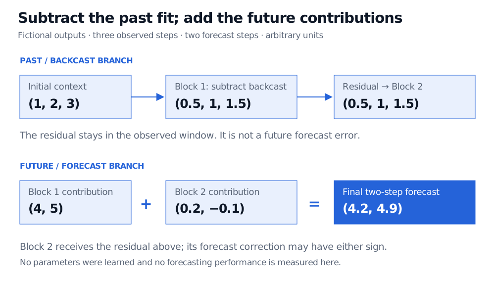
Take three observed inputs (1,2,3) in arbitrary units. Stipulate, rather than estimate, block 1's backcast (0.5,1,1.5). Subtraction leaves (0.5,1,1.5) for block 2.
Now stipulate two-step forecast components (4,5) and (0.2,−0.1). Their coordinatewise sum is (4.2,4.9). The second block raises the first forecast and lowers the second. A component need not be positive or equal to an observed value. These are arithmetic examples of the connections, with no fitted weights or measured accuracy.
Fictional block accounting: context (1, 2, 3) minus backcast (0.5, 1, 1.5) leaves residual (0.5, 1, 1.5) for block 2. Forecast components (4, 5) and (0.2, minus 0.1) sum to (4.2, 4.9). No model is fitted.
Original stipulated-output example in arbitrary units. Subtraction acts within the observed window; addition acts across the two future steps. The negative second-step contribution is permitted.
Decomposition depends on the basis
The original N-BEATS generic configuration learns its basis projections. The interpretable configuration constrains stacks to polynomial trend and Fourier seasonality bases. The coefficients remain learned. A labelled trend contribution is therefore a consequence of the chosen representation; it does not identify a true economic cause or prove the continuation of a market trend. See the original interpretability construction.
N-HiTS changes the resolutions
N-HiTS retains backcast subtraction and forecast addition, but changes how blocks process inputs and synthesize outputs:
Multi-rate input sampling: pooling compresses the observed input before the block's multilayer perceptron. Different pooling widths expose different effective resolutions.
Hierarchical interpolation: a block can predict fewer knot coefficients than there are horizon steps, then interpolate its contribution onto the full forecast grid. Across blocks, different interpolation granularities encourage coarse-to-fine specialization.
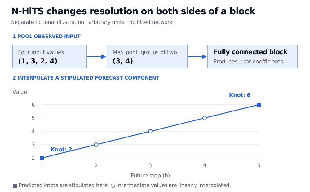
The original method uses max pooling. In a separate toy example, non-overlapping groups of two turn observed inputs (1,3,2,4) into (3,4). Separately, suppose a block supplies forecast knots of 2 at future step 1 and 6 at step 5. Linear interpolation fills the five-step component as (2,3,4,5,6). These future knots are stipulated predictions, not future data made available to the model.
Separate synthetic resolution example: max pooling observed inputs (1, 3, 2, 4) in pairs gives (3, 4). Stipulated forecast knots 2 at step 1 and 6 at step 5 produce linearly interpolated values 2, 3, 4, 5, 6. Squares are knots; hollow circles are intermediate values.
Original mechanism illustration in arbitrary units, separate from the residual-stack example. Pooling uses observed inputs. Output interpolation uses stipulated forecast coefficients, never observations from the future.
This coordinated input/output design distinguishes N-HiTS from simply renaming an N-BEATS stack. Coarse resolution can favour smooth components but can also miss sharp changes; it is an architectural bias, not evidence that financial shocks disappear.
Make the comparison about the forecast
Specify the target, observation frequency, lookback and forecast horizon before comparing architectures. A volume forecast and a return forecast answer different questions, even for the same instrument. A vector of point predictions also does not automatically supply a calibrated prediction interval.
Keep scaling, tuning and training within the information available at each forecast origin to avoid look-ahead bias. Compare against a suitable simple benchmark on identical later dates and horizons. The SelfMadeQuant Forecast Evaluation lesson develops rolling and expanding comparisons (public preview; full lesson requires membership). A smaller forecast error supports that evaluation result; trading value still depends on the decision, costs and stability.