Multilabel classification predicts which of several labels apply to the same observation, allowing none, one or several to be present. A quant's market-monitoring model might flag both high volatility and illiquidity for the same trading session. Forcing the session into one category would discard one of the conditions the desk wants to monitor.
The distinction from ordinary multiclass classification is the target definition. A multiclass, single-label task selects exactly one alternative from more than two classes. A multilabel task answers several yes-or-no questions. Labels can co-occur and can be statistically dependent; independence is not part of the definition. scikit-learn's classification guide makes this distinction explicit.
Two probabilities, two decisions
Consider a hypothetical model using information available at today's close to predict two conditions for the next session. Define the high-volatility and illiquidity labels using fixed measurement rules and the same forecast horizon. In that order, suppose the realised target is and the model's marginal probability estimates are
Each estimate concerns one label conditional on the available features. Their sum, 1.50, is valid: these are overlapping events, rather than competing outcomes. Separate sigmoid outputs are a common neural-network design. A single softmax over these two labels would impose a sum of one and would not represent both marginal probabilities correctly.
For illustration, choose a threshold of 0.50 for each label and predict 1 when its estimate is at least the threshold. Both predictions are then 1. This threshold is a decision rule, not a property of multilabel classification. False alarms and missed conditions can have different costs for each label; thresholds may therefore differ. Select them using validation data and an explicit objective, then evaluate on untouched test data. scikit-learn's threshold guide explains this separation between probability estimation and decisions.
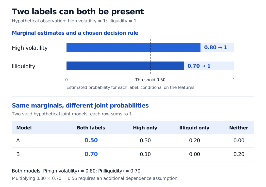
Original hypothetical example. Separate label probabilities need not sum to one. The joint-model rows show why the probability of both labels cannot be recovered by multiplying the two marginals without an additional assumption.
The lower panel matters if a risk process needs the probability of both conditions. Model A assigns probability 0.50 to both, 0.30 to high volatility alone, 0.20 to illiquidity alone and zero to neither. Model B assigns 0.70, 0.10, zero and 0.20 to those same outcomes. Both produce marginals of 0.80 and 0.70. Multiplying them gives 0.56 only under conditional independence of the labels given the features. Two marginal outputs alone do not establish that assumption.
What the training loss measures
A common objective adds binary cross-entropy across labels. For one observation with labels, true indicators and predicted probabilities , the unweighted sum is
For the observed target above, the negative-label terms vanish:
The logarithms are natural, and this is a sum over the two labels, not their average. Software may average instead; always check the reduction convention. PyTorch's loss documentation gives the labelwise expression and distinguishes sum from mean reduction.
Using this objective does not require the real labels to be independent. It scores the marginal predictions separately. Interpreting the same sum as the negative log-likelihood of the entire label vector under a product of Bernoulli distributions adds a factorized joint-model assumption. Good marginal forecasts can therefore coexist with an inadequate model of joint events. Methods that explicitly use label relationships, such as classifier chains, offer another modelling choice; their value must be tested against a simpler per-label baseline.
For the output-layer mechanics, Output Layers, Activation Functions, and Loss Functions compares sigmoid and softmax designs. The full lesson requires membership, with a public preview. Keep the distinction between separate marginal outputs and true label independence in mind when reading the recipe.
Evaluate the labels you might otherwise miss
Report performance per label before compressing it into one number. With class imbalance, an infrequent illiquidity flag can perform poorly while a common high-volatility flag dominates an aggregate result.
For F1 score, micro averaging pools true positives, false positives and false negatives across labels before calculating the score. Macro averaging calculates F1 for each label and then takes their unweighted mean, giving a rare label the same weight as a common one. Neither is universally preferable. Report label frequencies and state how undefined scores are handled when a label is absent from both targets and predictions. These averaging conventions are documented in scikit-learn's F1 reference.
Finally, preserve the forecast timeline. Future realised volatility can define a target, but it cannot be an input available today. Fit transformations and tune thresholds using past training and validation periods; reserve later observations for evaluation. If target windows overlap a split boundary, remove training examples whose outcomes would not yet be known at the test forecast time. A chronological splitter with an appropriate gap can help, but its gap must reflect label timing: ordering rows alone does not repair every form of leakage. See the TimeSeriesSplit documentation for its ordering and gap behaviour.
Sources
- scikit-learn: Multiclass and multioutput algorithms, sections 1.12.1–1.12.2
- PyTorch: BCEWithLogitsLoss, multilabel loss and reduction definitions
- scikit-learn: Tuning the decision threshold for class prediction
- scikit-learn: f1_score, averaging and zero-division conventions
- scikit-learn: TimeSeriesSplit, temporal ordering and gap parameter