Monte Carlo control is a family of reinforcement-learning methods that improves a policy using action values estimated from complete episodes. For a quant testing an execution rule, an episode might run from order arrival to a specified deadline: an early action is judged using the rewards that follow it through that deadline.
The learner needs sampled experience, not explicit transition probabilities. A simulator must still produce credible fills and costs; calling the learning algorithm model-free does not validate its environment.
Wait for the outcome, then assign the return
For an episode ending at time , define the return after action in state as
Here is the next reward and is the learning discount. The action value is the expected return from taking in and following policy afterwards. Estimate it by averaging the corresponding observed returns. This is the episodic Monte Carlo construction in Sutton and Barto, Chapter 5.
Consider a synthetic three-action episode with successive rewards 1, 2, 3, termination after the third reward, and :
These are returns from different times, not three independent observations of one action value. Suppose the pair occurs first at time zero, and its first-visit return in a separate episode is 3.23. Its two-sample estimate is . That is a reward estimate, not a 4.23% investment return.
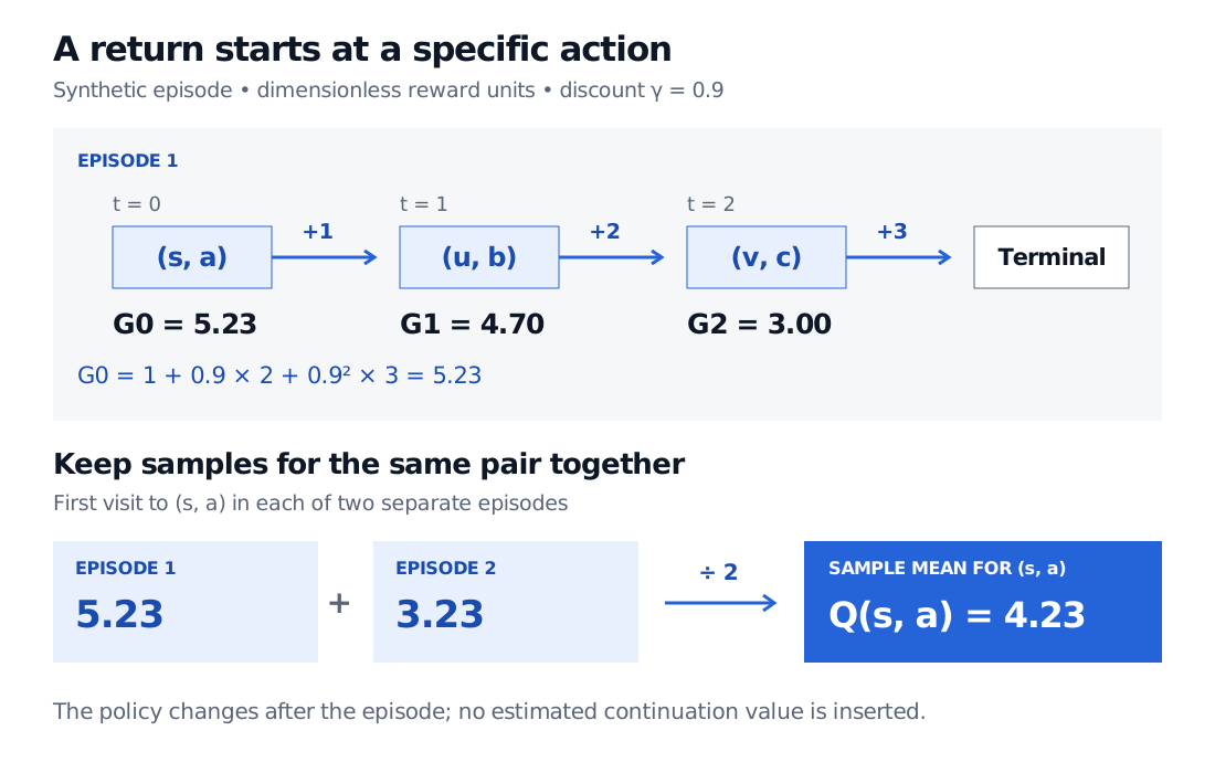
Original synthetic example, in dimensionless reward units. Average returns for the same state–action pair across episodes; do not average the three time-indexed returns as though they describe that one pair.
First-visit estimation uses only the earliest occurrence of each state–action pair in an episode. Every-visit estimation uses all occurrences, including repeats. For example, if the same pair occurs at both steps of a separate two-step episode paying 0 then 2, with discount 0.5, the two returns are 1 and 2. Starting with no previous observations, first-visit gives 1; every-visit gives 1.5. The repeated returns share an episode and are not independent samples. The CS234 policy-evaluation notes set out the two visit conventions.
Make the better-looking action more likely
Evaluation becomes control when the policy changes in response to the estimates. One on-policy first-visit procedure is:
- Generate a complete episode under the current exploratory policy.
- For each pair's first occurrence, add its return to that pair's sample mean .
- Make the next episode's policy epsilon-greedy with respect to the updated values.
For available actions and one selected greedy action, epsilon-greedy assigns it probability and each other action . With two actions and , these probabilities are 0.9 and 0.1, not 0.8 and 0.2: random exploration can also pick the greedy action. Such a policy is epsilon-soft because every action has probability at least .
The policy both generates experience and is improved, making this on-policy control. With fixed positive epsilon, exploration remains; the exact policy-improvement argument concerns the best policy within the epsilon-soft restriction. It does not say every noisy sample update improves performance. See Silver's model-free control lecture.
Claims of optimal convergence require more than “reduce epsilon.” In a stationary finite tabular episodic MDP with suitably bounded returns, check state–action coverage and the estimation scheme. Greedy in the limit with infinite exploration (GLIE) requires both infinitely many visits to the relevant pairs and an asymptotically greedy policy. An epsilon schedule alone does not establish visits to states that the starting conditions or dynamics never reach. These conditions are not a blanket guarantee for a neural-network trading agent.
What this changes in an execution experiment
Unlike temporal-difference learning, this Monte Carlo update uses the completed reward sequence, rather than bootstrapping from an estimated continuation value. It must wait for termination; long episodes can also produce noisy returns. A data cutoff is not automatically an economic terminal state. If the execution objective ends at a deadline, include time remaining in the state and account for residual inventory in the reward specification.
Historical orders generated by another policy are not automatically on-policy training episodes. Off-policy Monte Carlo methods need coverage and corrections such as importance sampling; simply pooling their returns can estimate the wrong policy's value.
For the policy-evaluation and improvement foundation, Markov Decision Processes and Value/Policy Iteration develops finite-state planning. Its public preview gives the outline; the full lesson requires membership.
Sources
- Sutton, R. S. and Barto, A. G., Reinforcement Learning: An Introduction, Chapter 5, §§5.1–5.4 and §5.5. This accessible copy is labelled “Second edition, in progress,” ©2014, 2015; it is a prepublication text. Read for complete-episode returns, visit conventions, control and epsilon-soft improvement.
- Silver, D., Lecture 5: Model-Free Control, sections “On-Policy Monte-Carlo Control,” “GLIE,” “MC vs. TD Control” and “Importance Sampling for Off-Policy Monte-Carlo.” Read for exploration, the control loop and the coverage/GLIE distinction. Numerical episodes and execution interpretation above are original illustrations.
- Homma, Y. and Brunskill, E., CS234 Notes — Lecture 3: Model Free Policy Evaluation, dated 20 March 2018, §§4.1, 4.3–4.5. Read for return/action-value notation, first/every-visit estimation, off-policy corrections and the Monte Carlo/TD distinction.