How TD learning updates a value estimate from one reward and the next estimate, with terminal-state handling, Monte Carlo comparison and convergence limits.
Temporal-difference learning
Temporal-difference (TD) learning updates an estimate of future cumulative reward using an observed reward and another current value estimate. In reinforcement learning, it lets a value learner improve after a single transition, before the final outcome is known. An execution simulator can therefore update its estimate of an inventory state's future net reward while the simulated order is still being worked.
The distinguishing feature is bootstrapping: part of the teaching target is itself an estimate. Sutton's 1988 paper formalised learning from differences between successive predictions.
One transition, one correction
Fix a policy π, meaning the rule used to choose actions. Its state value vπ(s) is expected discounted future reward from state s under that policy; V(s) is our current estimate. For a nonterminal transition, TD(0) uses
Here Rt+1 is the reward just observed, γ is the reward discount factor and αt is the learning step size. The TD errorδt measures the gap between the target and the old estimate. It is not the error against a known true value. TD(0) samples a transition rather than averaging over a known transition model. Barto's chapter slides distinguish this sampling from the model-based Bellman backup.
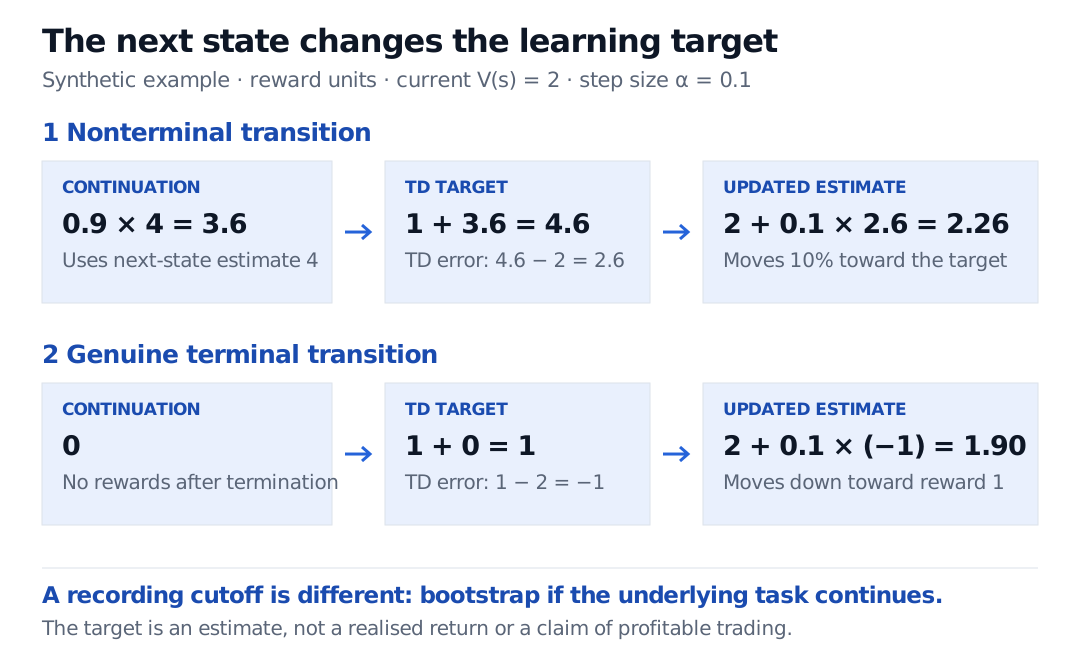
Take a synthetic transition with V(s)=2, reward 1, discount 0.9 and next-state estimate 4. The target is 1+0.9×4=4.6, so the error is 2.6. With α=0.1, the new estimate is 2+0.1×2.6=2.26. Only a tenth of the gap is closed; the estimate is not replaced by 4.6.
Synthetic TD updates start from value 2 with reward 1, discount 0.9 and step size 0.1. A nonterminal next-state estimate of 4 gives continuation 3.6, target 4.6, error 2.6 and updated value 2.26. A genuine terminal transition gives continuation 0, target 1, error minus 1 and updated value 1.90.
Original synthetic example in reward units. Both rows use the same current estimate and reward; only the continuation assumption changes.
If the next state is genuinely terminal, its continuation value is zero. With the same reward and old estimate, the target becomes 1 and the update becomes 2+0.1(1−2)=1.9.
A recording cutoff does not automatically mean termination. If the underlying task continues beyond a training window, retain the bootstrap from its final observed next state. A finite execution deadline that actually ends the defined task is different: include any final liquidation cost in the reward, then set continuation to zero. Remaining time belongs in the state when the policy's horizon matters. This follows the termination/truncation distinction in Farama's current guidance.
Why not wait for the realised return?
An episodic Monte Carlo value update waits for the complete discounted reward sum. TD(0) waits one step and supplies the missing future with V(St+1). For the fictional realised sequence of rewards 1,0,5, followed by termination, the Monte Carlo target at discount 0.9 is 1+0.9×0+0.92×5=5.05. The one-step TD target above was 4.6. Neither number is a guaranteed true expected value: one uses one realised path; the other uses an imperfect continuation estimate.
TD can learn from continuing tasks and propagate information without complete episodes, but bootstrapping introduces dependence on the quality of other estimates. It does not uniformly beat Monte Carlo. See Sutton and Barto, §§6.1–6.2.
Longer TD backups wait for several rewards before bootstrapping. TD(λ) combines horizons; eligibility traces carry a current TD error back to recently visited states. In tabular accumulating traces, the record for a state decays by γλ per transition and increases by one when that state is visited. At λ=0 this reduces to TD(0). Larger λ extends credit assignment; ordinary online traces should not be assumed exactly equivalent to every forward-return implementation. The textbook's §§7.1–7.3 develop these distinctions.
Prediction is not a trading policy
TD(0) above evaluates a fixed policy. Q-learning and Sarsa use TD targets for action values within control algorithms; an actor–critic method can use a TD error to train its critic. Updating a state value alone does not specify how actions improve.
A standard sufficient setting for tabular TD(0) convergence is a stationary finite Markov reward process induced by a fixed policy, an ergodic state chain, bounded rewards, discount below one, every state visited infinitely often, and positive per-state step sizes whose sum diverges while their squared sum converges. Under these conditions the estimates converge to that policy's values almost surely. A constant step size, such as the illustrative 0.1, does not satisfy those diminishing-step conditions. Hank Yang’s university notes, Theorem 2.1, state this tabular result. It does not guarantee convergence for an arbitrary neural trading system.
With shared function approximation, bootstrapping, off-policy learning and function approximation form the deadly triad: their combination can produce divergence. It does not imply every such algorithm diverges, and removing one ingredient is not a blanket guarantee for every remaining algorithm. Van Hasselt and colleagues examine both successful learning and unstable cases.
For finance, convergence within a simulator still concerns its rewards and dynamics. Omitting fees, impact or inventory penalties teaches a different objective; a stable value estimate cannot repair that modelling choice.
For the underlying recursion, the SelfMadeQuant lesson Markov Decision Processes and Value/Policy Iteration develops fixed-policy Bellman evaluation. Its preview is public; the full lesson requires membership.