A mixture of experts learns input-dependent weights or routes. Compare a soft blend with sparse top-one routing, then separate expert specialization, load balance and capacity.
Mixture of experts
A mixture of experts (MoE) combines several models, called experts, using a learned gate that makes their weights or selection depend on the input. For a quant, this offers a way to fit different predictive relationships in different parts of the feature space; sparse versions also let an input use only part of a larger model. Neither specialization nor a larger parameter count establishes better financial predictions.
The name predates large language models. Jordan and Jacobs’ original hierarchical model treats regression, classification and counting, with soft boundaries between regions. Experts can be simple statistical models; they need not be deep neural networks.
What the gate changes
For a normalized soft mixture with input x, expert outputs fi(x) and gate weights gi(x),
y(x)=i=1∑mgi(x)fi(x),gi(x)≥0,i=1∑mgi(x)=1.
The gate might apply softmax to learned scores. Unlike an equal-weight average, the combination can change from one input to another. Both the expert outputs and the gate depend on the input.
In a probabilistic MoE, the same idea combines conditional distributions: p(y∣x)=∑igi(x)pi(y∣x). A gate weight then describes mixture membership conditional on the input. It is not automatically the probability that an expert’s point forecast is correct. The training-time responsibility of an expert also uses the observed target; it differs from a gate computed from inputs alone.
Classical mixture estimation can use expectation–maximization. Neural MoE layers can instead train experts and the gate jointly by backpropagation. “Expert” names a component’s role, rather than independent training or statistical independence.
A blend of 5 or a selection of 6?
Take a stipulated regression example. At one input, expert A outputs 2 and expert B outputs 6; the gate assigns weights 0.25 and 0.75. All numbers are dimensionless, and the outputs are not estimated returns.
The soft mixture is 0.25×2+0.75×6=5. It lies between the two expert outputs, as a nonnegative weighted average must.
A hard gate chooses one expert. More generally, sparse top-k routing chooses only the k highest-scoring experts and can retain continuous weights among those selected. Unselected experts need not be evaluated. This is the conditional-computation mechanism in Shazeer et al.’s sparse MoE layer.
For this example’s top-one rule, renormalize the selected weight: B wins, its weight becomes 0.75/0.75=1, and the output is 6. This changes the prediction, not just the computation cost.
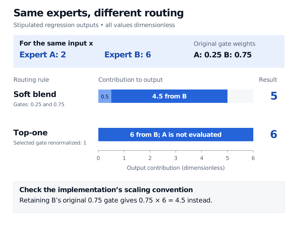
Two stipulated dimensionless expert outputs are A equals 2 and B equals 6, with original gate weights 0.25 and 0.75. The soft blend adds contributions 0.5 and 4.5 to give 5. Top-one routing with the selected gate renormalized to 1 gives 6. Retaining the original 0.75 gate would instead give 4.5.
Original stipulated regression example. Both rows use the same expert outputs and original gate weights. Selecting an expert and deciding how to scale its output are separate choices.
The scaling convention matters. A sparse implementation can retain the selected expert’s original gate weight. It would return 0.75×6=4.5 here. Switch Transformers, for example, multiplies its selected expert output by the router probability. Thus “top-one” alone does not specify the output formula. The renormalized calculation above is an explicit convention, not a universal sparse-layer rule.
Routing has a budget
A router can repeatedly favour a few experts. Those experts receive more training, reinforcing their advantage while others remain underused. Auxiliary balancing losses encourage broader use. Summed gate weights and counts of assigned inputs measure different things: equal weight totals need not mean equal workloads.
Expert capacity is also used to mean the number of inputs an expert can process in a batch. With fixed capacity, overloaded experts can cause overflow. Switch skips the affected expert computation and passes those token representations through a residual connection. Other designs need their own overflow policy. More buffer reduces overflow but consumes resources; sparse arithmetic savings also face routing and communication costs.
Specialization needs evidence
A learned expert need not correspond to a named market regime. Two experts may learn similar functions or unstable partitions, and a gate has no intrinsic temporal state-transition model. Calling components “calm-market” and “crisis-market” requires evidence beyond their routing frequencies.
For financial evaluation, fit both the gate and experts using information available at each historical decision. Later-known regime labels can introduce look-ahead bias. Compare the complete routed model with simpler alternatives on later data, and check routing concentration as well as predictive loss. A computational advantage in a language-model experiment is not evidence of profitable trading.