Mixed precision training uses lower precision for selected neural-network operations while retaining higher precision where numerical range or accuracy needs it. A quant training a large forecasting model may reduce activation memory and accelerate matrix operations on suitable hardware. The benefit depends on the workload; changing arithmetic does not establish that a forecast generalises.
The word mixed matters. Converting the entire model and every calculation to FP16 discards the safeguards that make the method useful.
Choose precision by job
FP16 and bfloat16 both store a scalar in 16 bits, compared with FP32's 32 bits, but they allocate those bits differently. Their floating-point arithmetic trades representable range against precision.
| Format | Exponent bits | Stored fraction bits | Consequence for training |
|---|---|---|---|
| FP16, IEEE binary16 | 5 | 10 | Relatively narrow range; small backward gradients can disappear. |
| bfloat16 | 8 | 7 | Much wider exponent range, comparable to FP32, but coarser spacing near a given normal value. |
| FP32, IEEE binary32 | 8 | 23 | More precision for sensitive calculations and parameter updates. |
The bfloat16 study by Kalamkar and colleagues, Section 3 and Table 1, explains this allocation. Wider range does not make bfloat16 uniformly more accurate than FP16.
Matrix products can use low-precision inputs with FP32 accumulation. Sensitive reductions and loss calculations may stay in FP32. In the historical Micikevicius et al. (2018) recipe, Sections 3.1–3.3, a separate FP32 master copy also receives weight updates, preserving small changes that could be lost when added directly to FP16 weights.
A duplicated master copy is not a universal requirement. In a common current PyTorch autocast workflow, model parameters remain FP32 while eligible operations use lower precision. Autocast selects operation types; the official AMP documentation advises against manually converting the model to half precision when using it. FP32 accumulation, FP32 parameter storage and the dtype of an operation's output are separate choices.
Scale before a small gradient disappears
FP16's largest finite value is 65,504. With gradual underflow, its smallest positive normal value is , while positive subnormal values extend down to . These are different boundaries. Underflow need not mean immediate zero at the normal boundary.
Consider a synthetic scalar gradient . In round-to-nearest, ties-to-even binary16 conversion, it rounds to zero: it is below . Multiplying that stored zero afterwards cannot restore the gradient.
Instead, multiply by before conversion. A CPU NumPy check, independently matched against exact rational decoding of binary16, gives:
| Calculation | Stored or recovered value |
|---|---|
| Cast directly to FP16 | 0 |
| Cast to FP16 | |
| Convert that result to higher precision, then divide by 1024 |
The middle value is a representable subnormal, equal to . The recovered number is nonzero but differs from the original by about 0.117%. Scaling has preserved a useful approximation, not eliminated rounding error.
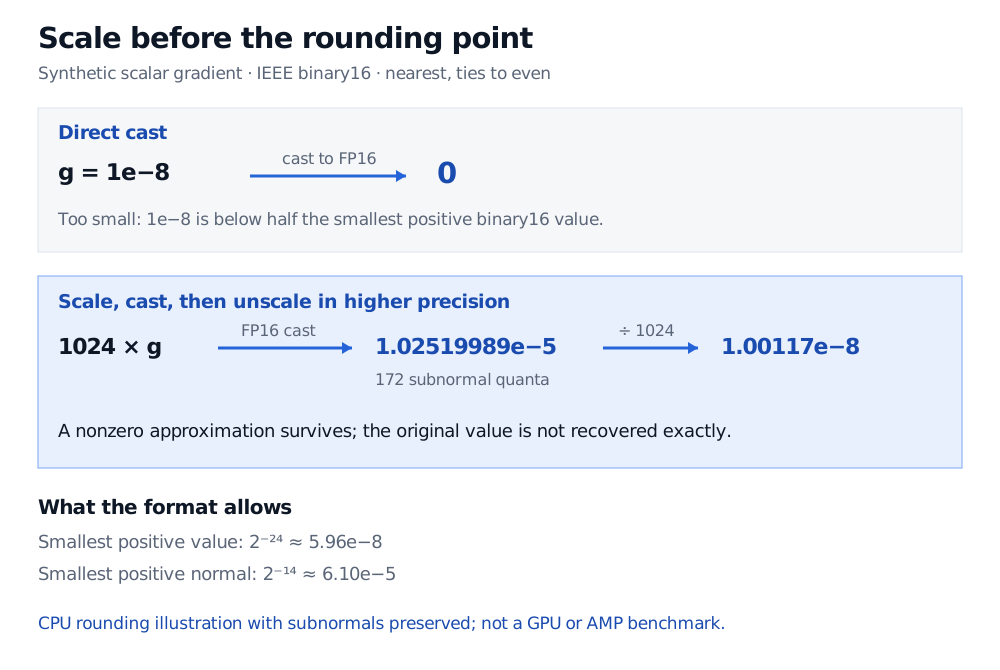
Original CPU rounding illustration with binary16 subnormals preserved. The two paths differ in when scaling occurs; this is not a GPU experiment or an AMP benchmark.
Actual training scales the loss before backpropagation, so intermediate backward gradients are enlarged before low-precision rounding occurs. With a positive scale held fixed for the step, the exact-arithmetic identity is
Divide parameter gradients by before the optimiser update. This is a change of numerical representation, not an intended increase in the learning rate. The original paper's Section 3.2 derives the mechanism. Our scalar cast illustrates one rounding point rather than simulating a complete backward pass.
Keep overflow and clipping in the right order
A scale large enough to protect tiny gradients can push large gradients into overflow. Dynamic loss scaling adjusts the scale: on detecting nonfinite gradients, PyTorch's scaler skips the affected optimiser step and reduces the scale; after a configured run of successful steps, it can increase it. A skipped update protects parameters but does not make the failed computation valid.
For ordinary FP16 AMP training, the official examples describe this sequence:
- Run the forward pass and loss with autocast's operation-specific precision.
- Scale the loss, then run backward outside the autocast context.
- Unscale parameter gradients before gradient clipping, so the threshold retains its intended units.
- Perform the scaler-controlled optimiser step, or skip it if gradients are nonfinite; update the scale for subsequent work.
If accumulating gradients over several mini-batches, keep a common scale until accumulation is complete, then unscale once for that optimiser's update. The training-workflow lesson explains the mini-batch and autograd machinery underneath this sequence. Its preview is public; the full lesson requires membership.
Loss scaling cannot repair forward overflow. If an activation or loss has already become infinite, scaling the loss afterwards cannot reconstruct it. A sensitive region may need FP32 arithmetic or a numerically safer formulation. The PyTorch AMP recipe's troubleshooting section suggests isolating autocast and scaling and running a suspected forward region in FP32.
Range is a format property; execution is a hardware policy
The scalar example assumes subnormals survive conversion. Hardware and kernels can instead flush subnormals to zero. For example, Cloud TPU's documented bfloat16 conversion uses nearest-even rounding and flushes bfloat16 subnormals. That policy is separate from both the format's exponent allocation and ordinary rounding to zero below the smallest subnormal.
Bfloat16's wider range often removes the need for FP16-style loss scaling; PyTorch's documented CPU bfloat16 example uses autocast alone. It still has rounding error and needs suitable operation choices.
Measure memory, training throughput and convergence against an FP32 baseline on the intended model and hardware. Optimiser state, retained FP32 parameters and other buffers mean 16-bit operations do not automatically halve total memory. CPU bottlenecks or small kernels may also leave little speed benefit, as the AMP recipe's performance discussion explains. In financial research, hold data splits and evaluation rules fixed while making that comparison: arithmetic efficiency and out-of-sample evidence answer different questions.
Sources
- Micikevicius et al. (2018), Mixed Precision Training, Sections 3.1–3.3: master weights, loss scaling and arithmetic precision.
- Kalamkar et al. (2019), A Study of BFLOAT16 for Deep Learning Training, Section 3 and Table 1: format comparison and mixed-precision data flow.
- PyTorch, Automatic Mixed Precision package, autocasting, gradient scaling and operation reference; stable documentation resolved to version 2.15 when checked on 1 November 2026.
- PyTorch, Automatic Mixed Precision examples, typical training, unscaled gradients, clipping and accumulation.
- PyTorch, Automatic Mixed Precision recipe, performance and nonfinite-loss troubleshooting.
- PyTorch,
GradScalersource documentation, dynamic scale adjustment and skipped optimiser updates. - Google Cloud, Improve your model's performance with bfloat16, format conversion details and TPU execution policy.