A minimum spanning tree (MST) connects every vertex in a connected, weighted, undirected graph without cycles and with the smallest possible sum of edge weights. For a network of trading sites, the weights could be the costs of leasing individual links. The MST gives the cheapest set of links that makes every site reachable.
A tree spanning vertices uses edges. Each weight can be a cost or a dissimilarity, with smaller values preferred. Kruskal's algorithm works with any finite real edge weights, including zero and negative values. A disconnected graph yields a minimum spanning forest, with one tree per connected component. Sedgewick and Wayne on weights and disconnected inputs
Join components in weight order
Kruskal's algorithm starts with each vertex in its own component. Visit edges from lightest to heaviest. Keep an edge when its endpoints are in different components, then merge those components. If its endpoints are already connected, the edge would close a cycle, so skip it. A disjoint set union tracks the components. On connected input, stop after accepting edges. Kruskal's original construction
Why is each merge safe? Separate one of the two components from the rest of the graph. No edge crossing that partition is lighter than the chosen edge. If an optimal tree that includes the earlier choices omits this edge, adding it creates a cycle with another crossing edge. Swapping out that other edge gives a spanning tree with all the earlier choices and no increase in total weight. With tied weights, a fixed tie order makes the result reproducible, but another order can produce a different tree of the same total weight. Sedgewick and Wayne on the cut property
The cheapest network can omit the cheapest route
In the fictional graph below, Kruskal takes A–B (1), B–C (2) and C–D (3). All four vertices are now connected, with a total cost of . The edges A–C (4), B–D (5) and A–D (9) remain outside the tree.
Now lower the weight of A–C from 4 to 2.5. Kruskal considers it before C–D, but A and C are already connected through B, so it skips A–C and still takes C–D. A shortest-path algorithm on the full graph would take the direct A–C edge at 2.5 instead of paying 3 via B. The spanning-tree objective counts each selected edge once across the whole network. The shortest-path objective counts only the edges on the route.
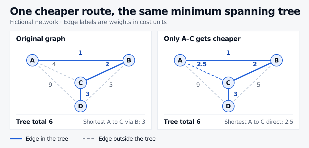
Lowering one edge weight changes the cheapest A-to-C route. The same three edges still give the cheapest network that connects all four vertices.
From return correlations to a market tree
To visualise which stocks move together, start with one edge per pair of assets. Compute the Pearson correlation from returns measured at the same frequency over a common set of dates, with nonzero sample variance for every series. Set the edge weight to so higher correlation gives a shorter edge. After centring each aligned return vector and scaling it to unit length, is the Euclidean distance between those vectors. Distinct assets with identical normalised vectors can therefore have distance zero. Pair-specific date sets can break the common-vector geometry even when the resulting weights can still be sorted. Bonanno et al. on the correlation-based tree
The tree reduces a dense network to links. It can reveal groups of stocks that tend to move together over the sample. A missing edge may still connect a highly correlated pair, and a near tie in the estimated correlations can change which edges survive when the sample changes. Tumminello et al. on sample uncertainty and filtered networks
The SelfMadeQuant lesson Minimum Spanning Trees: Kruskal and Prim compares both algorithms on another worked graph. The full lesson requires membership.
Sources
- Joseph B. Kruskal Jr. (1956), On the Shortest Spanning Subtree of a Graph and the Traveling Salesman Problem.
- Robert Sedgewick and Kevin Wayne, Minimum Spanning Trees, lecture slides for Algorithms, fourth edition.
- Giovanni Bonanno et al. (2004), Networks of Equities in Financial Markets, §2.
- Michele Tumminello, Fabrizio Lillo and Rosario N. Mantegna, Correlation, Hierarchies, and Networks in Financial Markets.