Minimum description length (MDL) selects an explanation by how compactly it describes both itself and the observed data under an agreed coding scheme, following the principle introduced in Rissanen’s 1978 paper. For a quant researcher, it makes extra factors, breakpoints or trading rules pay for the improvement they deliver in fit. A more elaborate model can still win: the question is whether it saves more data-description bits than it costs to describe.
The bill has two parts
The basic two-part MDL objective is
Here includes the selected structure and encoded parameter values. pays to communicate them; pays to reconstruct the data using that information. In regression, the second part may encode residuals, but it is a code length, not a residual count or unscaled squared error. This is a coding interpretation of regularisation. Grünwald's tutorial, §2.4, formalises the two terms.
Suppose two valid codebooks, fixed in advance, give the following lengths for the same fictional dataset, at the same recording precision. Any common side information is shared; all model-specific overhead is included.
| Candidate | Model description | Data given model | Total |
|---|---|---|---|
| A | 20 bits | 100 bits | 120 bits |
| B | 60 bits | 50 bits | 110 bits |
B spends 40 extra model bits and saves 50 data bits. Its total is 10 bits shorter, so MDL selects B. These are stipulated code lengths, not parameter counts. The example demonstrates the trade-off; it does not establish either model's forecasting performance.
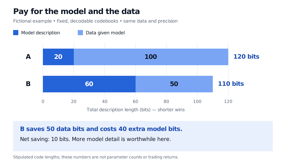
Original fictional comparison under fixed, decodable codebooks. Both bars describe the same data at the same precision; shorter total length wins.
What makes a number a code length?
A prefix code lets a decoder identify each message without needing an unpriced separator: no complete codeword starts another. The words
0, 10, 110 and 111 satisfy this rule. Their lengths, 1, 2, 3 and 3 bits, obey the Kraft inequality:The sum here is exactly 1. For nonnegative integer lengths, this condition characterises whether a binary prefix code exists. Arbitrarily awarding every candidate a tiny penalty need not define a valid code. Stanford's information-theory notes, §§1–2, explain this constraint and the distinction between ideal and integer lengths.
For a discrete outcome with probability , the ideal length is bits. A Shannon code can use bits. Thus gives exactly 3 bits, while gives about 1.585 ideal bits and a 2-bit Shannon codeword. Fractional ideal lengths are useful scoring quantities; they are not literal fractional binary symbols. Using instead gives nats: . Convert nats to bits by dividing by , and convert every term consistently.
Precision is part of the contract
A two-part code cannot communicate an arbitrary real coefficient exactly in finitely many bits. Specify a parameter grid or precision and pay for it; for example, selecting among 256 agreed grid values takes 8 fixed-length bits. Finer precision can improve fit while lengthening the model description. The coding convention matters, especially with small samples. See Grünwald, §§2.4.2–2.5.
For continuous data, a probability density is not a probability mass. As a concrete check, a uniform density of 2 on the interval from 0 to 0.5 assigns probability 0.02 to each bin of width 0.01. Its ideal bin code costs bits; applying the formula to the density alone gives , which is not a literal lossless message length. In density-based comparisons, use a common observation resolution and base measure; resolution terms cancel only when they are common to the candidates.
One principle, several constructions
Two-part coding is an accessible MDL construction, not its only form. Refined MDL can encode data through a universal distribution, including normalised maximum likelihood, without explicitly transmitting one fitted parameter vector first. Grünwald and Roos, §2.3, explain this distinction.
There is a precise connection to maximum a posteriori estimation: for discrete candidate models, if is proportional to and the conditional ideal length is , minimising their sum gives the same choice as maximising the posterior. This discrete correspondence does not identify all MDL methods with Bayesian inference. The Bayesian information criterion is related asymptotically to some MDL constructions under regular parametric assumptions; they need not agree in finite samples.
For financial prediction, compression is a selection criterion, not proof of profitable future trades. Dependence, changing regimes and a misspecified probability model can undermine the inference; even MDL can select poorly under misspecification, as Grünwald and Roos, §6.3, demonstrate. Keep preprocessing, model selection and final evaluation within a declared information schedule. Time-Ordered Train, Validation and Test Design develops that schedule and label-availability checks; its preview is public and the full lesson requires membership.
Sources
- Jorma Rissanen (1978), Modeling by shortest data description, IBM Research record, abstract: model-based compression for joint structure and parameter estimation.
- Peter Grünwald (2004), A Tutorial Introduction to the Minimum Description Length Principle, §§2.2 and 2.4–2.5: prefix codes, ideal lengths, two-part coding and parameter precision.
- Tsachy Weissman, Stanford EE376A/STATS376A, Lecture 6 (2018), §§1–2: Shannon lengths and Kraft–McMillan inequality.
- Peter Grünwald and Teemu Roos (2019), Minimum Description Length Revisited, §§2.2–2.3 and 6.3: refined MDL, asymptotic connections and misspecification.