Merton portfolio problem: Definition & Examples

The Merton portfolio problem asks how an investor should choose consumption and a portfolio through time to maximise expected utility. Its practical contribution is a rule for adjusting exposure as wealth and investment opportunities change, rather than choosing holdings once and leaving them untouched. In its familiar constant-opportunity, constant-relative-risk-aversion case, the optimal risky fraction stays constant even though the amount invested moves with wealth.

Merton’s original 1969 paper jointly studies investment and consumption, with a possible terminal bequest. The example below isolates the terminal-wealth investment problem: there is no consumption or labour income. That distinction matters because a consumption rule is another decision, not an automatic interpretation of the cash allocation. Merton (1969), §§II–IV and VII.

A portfolio policy, not a buy-and-hold weight

Let

S_t

be a risky asset following geometric Brownian motion, with known constant drift

\mu

and volatility

\sigma>0

\frac{dS_t}{S_t}=\mu\,dt+\sigma\,dW_t.

Here $W_t$ is Brownian motion. A risk-free account earns the continuously compounded rate $r$ . Write $X_t>0$ for wealth, $\pi_t$ for its risky fraction and $c_t$ for consumption per unit time. The budget equation is

dX_t=\left([r+\pi_t(\mu-r)]X_t-c_t\right)dt +\pi_t\sigma X_t\,dW_t.

The general consumption formulation values consumption along the way and possibly wealth left at $T$ . The numerical variant here instead sets $c_t=0$ and maximises $\mathbb{E}[U(X_T)]$ over admissible strategies that use information available at the time and preserve feasible wealth. Assume frictionless continuous trading, no taxes, no outside income, constant opportunities and no borrowing or short-sale restrictions.

Use constant relative risk aversion, or CRRA, preferences:

U(x)=\frac{x^{1-\gamma}}{1-\gamma},\qquad \gamma>0,\quad \gamma\ne1.

The limiting case

\gamma=1

uses

U(x)=\log x

. The coefficient is relative risk aversion:

-xU''(x)/U'(x)=\gamma

. Absolute risk aversion is

\gamma/x

, which falls as wealth increases. A larger

\gamma

means less tolerance for proportional wealth risk.

Where the constant fraction comes from

Let $V(t,x)$ be the best conditional expected terminal utility from wealth $x$ . The Hamilton–Jacobi–Bellman equation for this no-consumption variant is

0=V_t+\max_{\pi}\left\{ [r+\pi(\mu-r)]xV_x+ \frac12\pi^2\sigma^2x^2V_{xx}\right\}, \qquad V(T,x)=U(x).

The exposure rewards the marginal value of expected wealth growth and incurs a penalty through the negative curvature $V_{xx}$ . Differentiating the bracket with respect to $\pi$ gives

\pi^*=-\frac{\mu-r}{\sigma^2}\frac{V_x}{xV_{xx}}.

CRRA scaling and constant opportunities give $V(t,x)=A(t)x^{1-\gamma}/(1-\gamma)$ with $A(t)>0$ . Therefore $-V_x/(xV_{xx})=1/\gamma$ , so

\boxed{\pi^*=\frac{\mu-r}{\gamma\sigma^2}}, \qquad \text{cash fraction}=1-\pi^*.

This is the Merton fraction. The excess drift

\mu-r

rewards risk; relative aversion and variance reduce exposure. The denominator contains variance

\sigma^2

, not volatility

\sigma

. Holding the other inputs fixed, doubling volatility quarters the fraction, while doubling relative risk aversion halves it.

The dollar holding is

\pi^*X_t

. Thus unchanged preferences and opportunities imply the same percentage after a gain or loss, while the dollars at risk change. Rebalancing is needed to maintain that percentage; a fixed number of risky shares generally lets the fraction drift.

A fictional 37.5% policy

Take $\mu=0.08$ , $r=0.02$ , $\sigma=0.20$ and $\gamma=4$ , with time in years. These are stipulated model parameters, not estimates or an allocation recommendation. Then

\pi^*=\frac{0.08-0.02}{4(0.20)^2}=0.375.

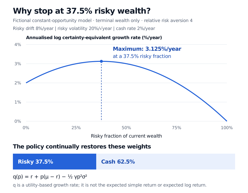
The policy continually maintains 37.5% risky wealth and 62.5% cash. At initial wealth of USD 100,000, that means USD 37,500 risky; at USD 200,000 it means USD 75,000 risky.

To see the trade-off, define the annualised log certainty-equivalent growth rate for a constant fraction $p$ :

q(p)=r+p(\mu-r)-\frac12\gamma p^2\sigma^2.

For this terminal CRRA problem, exact lognormal moments imply

U^{-1}\!\left(\mathbb{E}[U(X_T)]\right)=X_0e^{Tq(p)}.

Maximising expected utility therefore maximises

q(p)

. Its peak is

q(0.375)=0.03125

, or 3.125% per year. This quantity accounts for preferences; it is different from both mean return and mean log return.

Fictional terminal-wealth Merton model: with risky drift 8%, risky volatility 20% and relative risk aversion 4, annualised log certainty-equivalent growth peaks at 3.125% with 37.5% risky wealth and 62.5% cash.

Figure: Original fictional CRRA comparison. The curve maximises utility-based growth, and the allocation strip shows the continuously maintained risky and cash fractions.

Under the optimal policy, wealth itself follows

\frac{dX_t}{X_t}=0.0425\,dt+0.075\,dW_t.

The instantaneous expected-return drift is 4.25% per year, and the annualised diffusion volatility is 7.5%. The expected log-growth rate subtracts the Itô correction:

\frac{\mathbb{E}[\log(X_T/X_0)]}{T} =0.0425-\frac12(0.075)^2=0.0396875.

For one year, the expected simple return is instead

\mathbb{E}[X_1/X_0-1]=e^{0.0425}-1 \approx 4.3416\%.

Calling 4.25% the exact expected one-year simple return would mix an instantaneous model coefficient with a finite-horizon return.

What breaks the shortcut

The absence of $x$ or $T-t$ from the fraction is a consequence of this specification. It is not a general claim that wealth, age or horizon never affect portfolio choice. CRRA scaling removes wealth from the risky percentage, and constant investment opportunities remove the motive to hedge their future changes. Changing terminal preferences, income or constraints can change that result.

If returns, volatility or interest rates depend on stochastic state variables, future opportunities become a source of risk. Optimal demand can then include intertemporal hedging as well as the current risk-premium exposure: assets may help offset adverse changes in the opportunities available later. Simply inserting today’s

\mu_t,r_t,\sigma_t

into the constant-fraction formula can miss this term. Merton derives this demand decomposition in his 1973 paper, §5, especially equation (16) and pp. 876–877; the equilibrium extension is the intertemporal CAPM.

The unconstrained formula can also produce a negative fraction or one above 100%, implying short selling or borrowing. A constrained problem must impose its actual trading limits. In the one-risky-asset constant-opportunity case with the sole restriction $0\le\pi\le1$ , the concave objective’s optimum is the unconstrained fraction clipped to that interval. Costs of repeated trading require a different control problem.

For the related static allocation calculation, Mean-Variance Optimisation derives the with-cash solution from excess returns and a covariance penalty. Its public preview outlines the lesson; full teaching requires membership. The algebra resembles Merton’s fraction, while the Merton problem derives a trading policy from an explicit intertemporal utility objective.

Sources

Merton, “Lifetime Portfolio Selection under Uncertainty: The Continuous-Time Case” (1969), §§II–IV and VII: wealth dynamics, consumption/bequest objective, CRRA solution and constant-share interpretation. The paper uses a different symbol convention for utility curvature.
Merton, “An Intertemporal Capital Asset Pricing Model” (1973), original paper text, §5, pp. 875–877: state-dependent opportunities and hedging demand; §6, pp. 877–878: constant-opportunity special case.
Penati and Pennacchi, Finance 400 notes on Merton’s intertemporal model, §§I–II, pp. 1–4: state-variable budget equation, first-order conditions and interpretation of the hedging component.

A portfolio policy, not a buy-and-hold weight

Where the constant fraction comes from

A fictional 37.5% policy

What breaks the shortcut

Sources

Related terms

Expected utility and risk aversion

Geometric Brownian motion

Rebalancing