Menchero optimised linking: Definition & Examples

Menchero optimised linking combines single-period arithmetic attribution effects into contributions that sum to the difference between compounded portfolio and benchmark returns. It uses a common scale plus the smallest squared period corrections needed for reconciliation. A performance report can therefore explain the whole horizon without leaving a compounding residual.

The inputs are already-computed performance attribution effects. Linking does not identify the investment decisions or establish manager skill. “Optimised” describes the adjustment of reporting coefficients; it does not mean minimising economic risk or choosing an optimal portfolio.

A report that fails to add up

Consider two fictional periods, with returns measured consistently and no external cash flows. Effects A and B are illustrative components, each expressed as a contribution to arithmetic active return.

Period	Portfolio	Benchmark	Effect A	Effect B	Active return
1	10%	5%	+3 pp	+2 pp	+5 pp
2	−5%	−2%	−1 pp	−2 pp	−3 pp

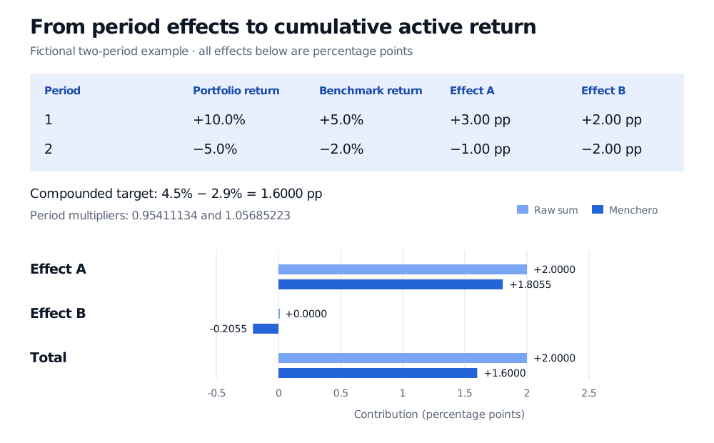
Each row reconciles. The columns summed through time give A = 2 percentage points and B = 0. Yet the portfolio compounds to

1.10(0.95)-1=4.5\%

, and the benchmark to

1.05(0.98)-1=2.9\%

. The cumulative arithmetic difference is 1.6 percentage points, rather than the 2 points from adding the period differences.

Scale first, then reconcile

Let $r_{p,t},r_{b,t}$ be decimal returns over $n$ subperiods, and let $e_{j,t}$ be effect $j$ , with $\sum_j e_{j,t}=d_t=r_{p,t}-r_{b,t}$ . Define

R_p=\prod_{t=1}^{n}(1+r_{p,t})-1,\qquad R_b=\prod_{t=1}^{n}(1+r_{b,t})-1,\qquad \Delta=R_p-R_b.

For positive gross returns, the Menchero scale is

M=\frac{\Delta}{n\left[(1+R_p)^{1/n}-(1+R_b)^{1/n}\right]}.

Apply a common period multiplier $w_t=M+a_t$ to every effect in that period:

E_j=\sum_{t=1}^{n}w_t e_{j,t},\qquad a_t=\frac{\left(\Delta-M\sum_{s=1}^{n}d_s\right)d_t} {\sum_{s=1}^{n}d_s^2}.

These are the scale and correction equations in Menchero’s primary technical disclosure, with notation changed. Eagle’s documentation describes the same scale-then-correct procedure. The result satisfies

\sum_j E_j=\Delta

whenever the input rows reconcile.

Why this correction? Put

c=\Delta-M\sum_t d_t

. Reconciliation requires

\sum_t a_td_t=c

. Minimise

\frac12\sum_t a_t^2

subject to that constraint. The Lagrangian

\mathcal{L}=\frac12\sum_t a_t^2-\lambda\left(\sum_t a_td_t-c\right)

gives $a_t=\lambda d_t$ and hence $\lambda=c/\sum_t d_t^2$ . This proves the stated minimum for fixed $M$ and nonzero $\sum_t d_t^2$ . The objective concerns distance from the chosen common scale, not an effect’s volatility, statistical uncertainty or economic importance.

For the example,

M\approx1.01832439

. Scaling the raw total alone would give

1.01832439(0.02)=0.02036649

, leaving a required correction of about −0.436649 percentage points. The adjustments are

a_1\approx-0.06421306

and

a_2\approx0.03852783

Linked contribution	Calculation in decimal returns	Percentage points
A	$0.95411134(0.03)+1.05685223(-0.01)$	+1.805482
B	$0.95411134(0.02)+1.05685223(-0.02)$	−0.205482
Total	A + B	+1.600000

Values use unrounded coefficients. Effect B’s raw sum was zero, but its positive and negative observations receive different multipliers. Its linked contribution can therefore be nonzero.

Fictional two-period example: raw A is 2 percentage points and B zero; Menchero gives A 1.8055 and B minus 0.2055, summing to the compounded difference of 1.6000 points.

Original fictional example. One multiplier per period applies to both effects; the linked total matches the difference between compounded returns.

Equal cumulative returns still need checking

When $R_p=R_b=R$ , use the continuous limit

M=(1+R)^{(n-1)/n}.

Do not automatically set $a_t=0$ . Take portfolio returns of 10%, 10% and benchmark returns of 21%, 0%. Both compound to 21%, so

\Delta=0

and

M=1.1

. However,

d_1=-0.11

d_2=0.10

and

\sum_t d_t=-0.01

. Leaving the adjustments at zero would report −1.1 percentage points, despite equal final returns. The correction numerator is

0-1.1(-0.01)=0.011

, so the correction remains necessary. The resulting multipliers are about 1.04524887 and 1.14977376, and their weighted active returns sum to zero.

The separate case

d_t=0

in every period makes

\sum_t d_t^2=0

. Then portfolio and benchmark paths coincide, reconciliation is already satisfied, and choose

a_t=0

. Individual effects can still offset each other within a period; they need not vanish.

For numerical work near cumulative equality, set $x=(1+R_p)^{1/n}$ and $y=(1+R_b)^{1/n}$ . The algebraically equivalent expression

M=\frac1n\sum_{k=0}^{n-1}x^{n-1-k}y^k

avoids subtracting nearly equal roots and includes the equality limit. Retain the correction and check the final residual. The displayed formula documentation in R-Finance’s implementation agrees with the general formula, but the inspected code sets the adjustment to zero whenever cumulative returns are equal. The counterexample above shows why that branch is insufficient.

Interpreting the linked result

Cariño linking uses different coefficients and can allocate the same reconciled total differently. Record the linking convention alongside the attribution model. Reconciliation alone does not make one explanation uniquely economically correct.

This is an arithmetic decomposition of $R_p-R_b$ . Geometric attribution instead works with relative wealth, $(1+R_p)/(1+R_b)$ , and a different aggregation structure. Keep the benchmark, return basis, subperiod grid and treatment of costs consistent before comparing reports. The formulas here assume returns greater than −100%; a total-loss observation needs explicit treatment rather than blindly applying roots and limits.

For the return measurement underneath the calculation, see Risk-Adjusted Performance Measures, especially its time-weighted compounding section. The preview is public; the full lesson requires membership.

Sources

Jose G. Menchero (2000), An Optimized Approach to Linking Attribution Effects Over Time, The Journal of Performance Measurement, Fall, 5(1), pp. 36–42. The publisher’s abstract was accessible; the full paper is sold separately and was not read for this article.
Jose Gabriel Menchero, US7246091B1, Method and system for multi-period performance attribution, “Multiple-Period Arithmetic Attribution,” equations 10–20. Primary technical disclosure used for the derivation and limit.
Eagle: Menchero Multiple-Period Smoothing, “Arithmetic Smoothing Calculation” and calculation steps.
Andrii Babii, R-Finance PortfolioAttribution, Menchero.R, formula documentation and cumulative-equality code branch, inspected 30 October 2026.

A report that fails to add up

Scale first, then reconcile

Equal cumulative returns still need checking

Interpreting the linked result

Sources

Related terms

Active return

Cariño linking algorithm