Maximal information coefficient: Definition & Examples

The maximal information coefficient (MIC) measures association by searching rectangular grids for a large normalized mutual information score. A quant can use it to flag nonlinear relationships that Pearson correlation misses, then investigate their shape and stability. A high score alone does not establish a tradable signal.

Let the grid follow the relationship

For paired data $D=\{(x_i,y_i)\}_{i=1}^n$ , choose a grid $G$ with $k$ columns and $\ell$ rows. Write $p_{ab}$ for the fraction of observations in cell $(a,b)$ and $p_{a\cdot},p_{\cdot b}$ for its marginal fractions. The grid's mutual information is

I_G=\sum_{a,b:p_{ab}>0}p_{ab}\log\frac{p_{ab}}{p_{a\cdot}p_{\cdot b}}.

The original finite-sample criterion is

\operatorname{MIC}_B(D) =\max_{\substack{k,\ell\ge2\k\ell<B(n)}} \max_{G\in\mathcal{G}_{k,\ell}} \frac{I_G}{\log\min(k,\ell)},

where

\mathcal{G}_{k,\ell}

contains the grids of that size. Their cuts need not be equally spaced. The denominator bounds the normalized score between zero and one; use the same logarithm base in numerator and denominator. The budget

B(n)

limits the number of cells searched. The 2011 paper commonly uses

B(n)=n^{0.6}

and the strict inequality shown here. Reshef et al. (2011)

The search asks whether some partition exposes dependence, rather than whether one straight line fits. MIC is symmetric and unsigned: it cannot tell you whether increasing a feature raises or lowers the response.

Zero correlation, perfect separation

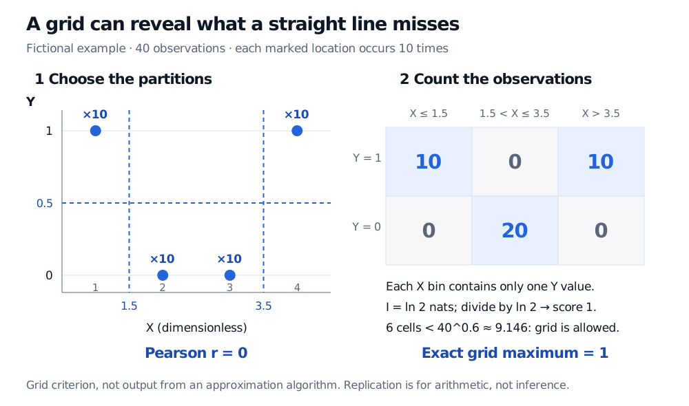
Construct 40 fictional observations: each pair $(1,1)$ , $(2,0)$ , $(3,0)$ and $(4,1)$ occurs ten times. Both variables are dimensionless. Their means are $\bar x=2.5$ and $\bar y=0.5$ . The four distinct centered cross-products are $-0.75$ , $0.25$ , $-0.25$ and $0.75$ . Their sum is zero, so the sample Pearson correlation is exactly zero despite the deterministic relationship.

Cut $X$ at 1.5 and 3.5, and $Y$ at 0.5. The resulting counts are:

$X$ bin	$Y=0$	$Y=1$
$X\le1.5$	0	10
$1.5<X\le3.5$	20	0
$X>3.5$	0	10

Each column identifies $Y$ perfectly, and the two $Y$ values have equal frequency. Every occupied cell has $p_{ab}/(p_{a\cdot}p_{\cdot b})=2$ . Thus, using natural logarithms,

I_G=\left(\tfrac14+\tfrac12+\tfrac14\right)\ln2=\ln2, \qquad \frac{I_G}{\ln\min(3,2)}=1.

This grid has six cells, and

6<40^{0.6}\approx9.146

. It is admissible and attains the universal upper bound, proving the exact grid criterion equals one for this dataset and budget. For comparison, the best

2\times2

partition scores only about

0.3113

: the third

X

bin lets the grid separate the two outer groups from the middle.

Forty fictional observations occupy (1,1), (2,0), (3,0) and (4,1), ten times each. Pearson correlation is zero. X cuts at 1.5 and 3.5 and a Y cut at 0.5 yield six cells with counts 10, 0, 10 in the upper row and 0, 20, 0 below; normalized mutual information is one.

Original fictional example, with dimensionless variables. The six-cell grid fits within the declared sample-size budget; the perfect score is an exact grid result, not an approximation-library output.

The replication matters to the stated grid budget. With only the four distinct observations,

4^{0.6}\approx2.297

, so the six-cell grid is excluded. Even minepy's minimum budget of four would exclude it. Repeating points supplies this arithmetic example with 40 records; it does not supply 40 independent pieces of evidence.

An exact statistic and a computed score are different objects

The example proves a mathematical maximum without running a general MIC algorithm. Practical software searches are constrained approximations. The original APPROX-MIC procedure is distinct from $\operatorname{MIC}_e$ , a later efficiently computable estimator of the population quantity

\operatorname{MIC}_*

; these names are not interchangeable. The 2016 follow-up separates dependence-strength estimation from independence testing.

For example, minepy's documented API selects mic_approx or mic_e through the estimator argument; its mic() method can therefore return different statistics. Report the estimator, library version, sample size and grid/search settings alongside a numerical score. Do not label the hand-calculated value above as output from either implementation.

Use the score to open a research question

MIC was motivated partly by equitability: giving similar scores to equally noisy relationships with different shapes. This is a goal that needs a specified definition, noise model and relationship class. Kinney and Atwal challenged the original formulation and simulation evidence. Later work developed a more formal framework and new estimators. A MIC value should not be read universally as “the fraction of variance explained,” or as proof that all nonlinear relationships are ranked fairly.

The same maximization that finds an interesting grid can exploit sample noise. Larger grid budgets permit more flexibility; finite-sample scores need calibration rather than a universal cutoff. Searching many feature pairs also creates data-snooping risk. The MINE authors' significance guidance explicitly calls for addressing multiple testing. In financial time series, any null calibration must also respect the dependence structure being assumed; unrestricted shuffling is not automatically valid for serially dependent data.

Inspect the scatterplot, check data timing and shared drivers, and evaluate any resulting predictive hypothesis on later data. Association alone does not establish causality, forecast stability or performance after trading costs. The usual return-signal information coefficient, often a correlation between a signal and subsequent returns, is a separate concept.

For the linear baseline, Basic Statistics and Regression develops sample correlation, fitted lines and the limits of in-sample fit. Its public page is a preview; the full lesson is available with a free signed-in account.

Sources

Reshef et al. (2011), Detecting Novel Associations in Large Data Sets, pp. 1518–1519: original characteristic matrix, normalization and grid budget.
minepy 1.2.6, Python API: estimator choices and budget/search parameters.
Kinney and Atwal, Equitability, mutual information, and the maximal information coefficient: the equitability critique and finite-grid overfitting discussion.
Reshef et al. (2016), Measuring Dependence Powerfully and Equitably: population MIC, $\operatorname{MIC}_e$ and the distinction between equitability and testing power.
MINE, Technical Information: multiple-testing guidance.

Let the grid follow the relationship

Zero correlation, perfect separation

An exact statistic and a computed score are different objects

Use the score to open a research question

Sources

Related terms

Correlation