How Isomap estimates curved-surface distances with a neighbourhood graph, why graph distance differs from a true geodesic, and where financial maps can fail.
Manifold learning and Isomap
Manifold learning is nonlinear dimensionality reduction based on the idea that observations with many recorded features may lie on, or near, a lower-dimensional curved surface. For a quant researcher, it offers a way to explore nonlinear similarities among assets or market states. The result depends on whether the chosen features and distances describe a meaningful geometry; a compact map does not establish a forecasting signal.
A manifold looks approximately flat in a sufficiently small neighbourhood. A circle, for example, is locally one-dimensional even though its points have two Cartesian coordinates. Manifold methods try to recover aspects of that hidden structure. They preserve different things: Isomap targets estimated distances along the surface, while t-SNE matches neighbourhood affinities. The scikit-learn manifold guide introduces this nonlinear approach.
Isomap: use local hops to estimate a global distance
Isomap, short for isometric mapping, replaces direct pairwise distances with shortest-path distances through a neighbourhood graph, then applies classical multidimensional scaling (MDS).
Connect nearby observations. Use a radius or nearest-neighbour rule. Give each graph edge the original distance between its endpoints; treat the graph as undirected.
Find shortest paths. Sum edge lengths along candidate routes and retain the minimum for each pair. These graph distances estimate manifold geodesics: shortest paths constrained to the underlying surface.
Fit coordinates with classical MDS. Embed the graph-distance table in the chosen dimension through an eigendecomposition.
These are the three stages in Tenenbaum, de Silva and Langford (2000), Table 1. There are two separate approximations: the graph estimates unknown surface distances, and the Euclidean embedding approximates the graph geometry. Neither step promises exact preservation for arbitrary data or a chosen small dimension.
Four points, three answers
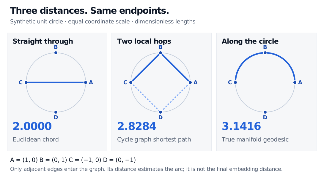
Take four synthetic points on a unit circle, in dimensionless coordinates:
A=(1,0),B=(0,1),C=(−1,0),D=(0,−1).
Connect only adjacent points around the cycle: A–B, B–C, C–D and D–A. Each edge has Euclidean length 2. Between opposite points A and C:
Distance definition
Calculation
Length
Direct Euclidean chord
Straight from A to C
2
Shortest path in this graph
A–B–C or A–D–C
22≈2.8284
True circle geodesic
Either semicircle, radius one
π≈3.1416
Opposite unit-circle points A=(1,0) and C=(-1,0) have Euclidean chord length 2, adjacent-edge cycle graph distance 2 square root of 2, approximately 2.8284, and true circle arc length pi, approximately 3.1416.
Original synthetic unit-circle geometry. The graph contains four adjacent chords, each of length square root of 2. The highlighted upper route and the lower route tie; graph distance is an estimate of the arc, not a final embedding distance.
The graph avoids the direct A–C chord, but its two retained chords still cut inside the circle. Calling 2.8284 the exact circle geodesic would be wrong. Adding sufficiently dense samples with appropriately local edges can improve the approximation. Adding an A–C edge instead immediately reduces this graph distance to 2, creating a shortcut through the circle’s interior.
The circle also illustrates a different limit: intrinsic dimension one does not mean that all circular distances can be preserved on a straight line. A single angular coordinate needs a cut, and ordinary line distance fails across that cut. This example checks the distance-estimation stage; it is not a claim that Isomap perfectly unrolls a closed circle into one Euclidean dimension.
The neighbourhood rule is a modelling choice
Too few edges can disconnect the graph, leaving infinite distances between components. Too many can bridge separate folds and destroy the intended geometry. A connected graph alone is therefore insufficient. Inspect its edges and components, and check whether conclusions survive reasonable changes to neighbourhood size and feature scaling. The original paper, pp. 2321–2322 and notes 18–19 ties approximation quality to sampling density, curvature and separation between branches; its asymptotic result is not a finite-sample guarantee for market data.
For an asset map, decide whether proximity should reflect raw returns, volatility-normalised returns or other economically chosen features. A volatility-dominated distance and a standardised distance answer different questions. Noise, sparse observations and changing market structure can alter neighbours and therefore many shortest paths. These are reasons to inspect the original observations before interpreting plotted groups as stable economic categories.
Placing tomorrow’s observation
The original algorithm constructs coordinates for its supplied sample. Applying a fitted map to a new observation requires an extension. Scikit-learn’s Isomap transform method connects new observations to training neighbours, estimates distances through the training graph and projects the resulting kernel onto the fitted embedding. It does not guarantee reliable placement far from the training geometry. Refitting on an enlarged sample can move earlier coordinates.
For a historical forecasting experiment, fit scaling, neighbourhoods and the embedding using only the information available in each training window. Keep later observations out of those choices; an unsupervised graph can still introduce look-ahead bias. Then evaluate any downstream forecast on later held-out data. This applies the training-only preprocessing principle to the whole representation pipeline.