How loss landscapes and Hessian sharpness describe parameter sensitivity, why equivalent models can look differently sharp, and how to read a two-dimensional slice.
Loss landscape and sharpness
A loss landscape is the loss function viewed across a model's parameter space, with the data and evaluation procedure held fixed. Sharpness describes how much the loss rises under a specified perturbation of those parameters. For a quant forecasting model, this geometry can help diagnose sensitive training updates; it cannot establish whether forecasts will survive a future market regime.
A landscape plot and a training-loss curve answer different questions. The first varies parameters; the second follows the particular sequence of parameters visited during training. Neither is an out-of-sample performance result.
What does “sharp” measure?
A small perturbation can mean a fixed Euclidean distance, a relative change in each weight, or a change scaled separately within each network filter. These are different experiments. A sharpness comparison needs to name the perturbation size, directions and scaling convention.
At a smooth stationary minimum θ⋆, the Hessian matrix H=∇2L(θ⋆) gives the local quadratic approximation
L(θ⋆+δ)−L(θ⋆)≈21δTHδ.
For a unit direction v, the directional curvature is vTHv. A large positive eigenvalue identifies a direction with a rapid local loss increase under the chosen coordinate scale. A minimum can be steep in one direction and flat in another. This local approximation does not describe an arbitrarily large neighbourhood, and a zero eigenvalue need not imply an exactly constant-loss path.
Two parameter vectors, one prediction function
Consider an analytic toy model with two scalar weights,
fw1,w2(x)=w1w2x.
Fit the single observation (x,y)=(1,1) using unpenalised squared error:
L(w1,w2)=(w1w2−1)2.
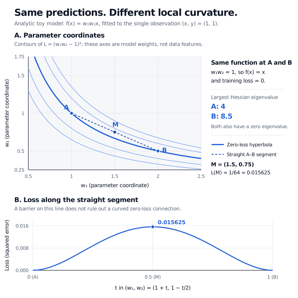
This deliberately small example exposes a coordinate issue; it is not a fitted financial model. The parameter vectors A=(1,1) and B=(2,0.5) both give f(x)=x for every input, with training loss zero. Their Hessians are nevertheless different:
HA=(2222),HB=(0.5228).
Their eigenvalues are respectively (0,4) and (0,8.5). Ranking the two weight vectors by the largest Hessian eigenvalue calls B sharper, although the prediction function is unchanged. Generalisation cannot differ between these two functions on the same prediction task, because their predictions are identical.
Analytic toy loss: A at (1,1) and B at (2,0.5) both have loss zero and define the same prediction function. Their largest Hessian eigenvalues are 4 and 8.5. The straight midpoint (1.5,0.75) has loss 0.015625, while the curved hyperbola joining A and B has loss zero.
The axes in panel A are parameter coordinates. Panel B evaluates the loss only along the straight segment between A and B; a barrier on that segment does not establish separate basins.
The straight midpoint is M=(1.5,0.75), giving
L(M)=(1.5×0.75−1)2=641=0.015625.
Yet the curved path (w1,w2)=(a,1/a), with 1≤a≤2, connects the same endpoints with loss exactly zero throughout. A straight interpolation therefore finds a barrier that a curved path avoids. These are not two disconnected minima.
The example also separates weight stability from prediction stability. Multiplying one weight by a positive factor and dividing the other by the same factor changes the weight coordinates without changing the model. Dinh et al. (2017) establish related rescaling counterexamples for rectified neural networks: common flatness measures can change while the represented function stays fixed. Raw parameter-space flatness is therefore not a generalisation certificate.
Read the slice before reading the valley
A real neural network can have millions of parameters. A two-dimensional figure usually evaluates a slice such as
L(θ⋆+αd1+βd2),
where d1,d2 are chosen parameter directions. Its axes are coefficients of those directions, not a complete map of the landscape. A calm-looking slice can miss steep or nonconvex directions elsewhere.
Li et al. (2018) use filter-wise normalisation: each filter's perturbation direction is scaled to the norm of the corresponding trained filter. This addresses weight-scale effects in their visual comparisons. Their experiments find sharpness–generalisation associations under that protocol; the normalisation does not turn every slice or Hessian statistic into a universal measure of generalisation.
For a useful comparison, keep the loss definition, data sample, parameterisation, plot scales and model evaluation mode explicit. Specify how regularisation and normalisation state enter the evaluation. Then check prediction performance on the appropriate held-out data. A lower training loss, a wider valley and a better chronological validation score are separate observations; a picture alone does not identify which mechanism caused the score difference.
Reading Loss Curves develops the complementary workflow: log experiments, distinguish training failures from overfitting, and select configurations using validation data. Its preview is public; the full lesson requires membership.
Sources
Dinh, L., Pascanu, R., Bengio, S. and Bengio, Y. (2017), Sharp Minima Can Generalize For Deep Nets, Sections 2–4.2: definitions, equivalent parameterisations and Hessian-based measures.
Li, H., Xu, Z., Taylor, G., Studer, C. and Goldstein, T. (2018), Visualizing the Loss Landscape of Neural Nets, Sections 3–5: interpolation, two-dimensional slices and filter-wise normalisation.