A latent diffusion model generates in a learned representation, then decodes to data space. Separate compression, denoising and financial scenario validity.
Latent diffusion model
A latent diffusion model (LDM) learns to generate data by denoising a learned latent representation and decoding the result into the original data space. For a quant considering synthetic market scenarios, the attraction is doing repeated denoising in a smaller representation; the critical question is whether that representation retains the financial events the scenarios must reproduce.
A representation model plus a generative model
In the original image method, an autoencoder first learns an encoder E and decoder D. Spatial compression makes the latent representation cheaper to process. A diffusion network then learns its distribution, and the decoder maps generated latents back to images. Conditioning can enter through concatenation or cross-attention, for example to guide generation with text. These are separate roles: compression, generation and control. Rombach et al., §§3.1–3.3.
The authors' implementation freezes the first-stage autoencoder during diffusion training. Its latent handling can include posterior sampling and a scale factor; the decoder reverses that scaling. Thus a real model's latent coordinates need not be a deterministic, unscaled encoder output. CompVis, LatentDiffusion.
Use z0 for a clean latent. In a noise-prediction formulation, a training example is corrupted as
zt=αˉtz0+1−αˉtϵ,ϵ∼N(0,I).
Here I is the identity covariance, and αˉt=∏j=1t(1−βj) is cumulative signal retention for forward noise variances βj. The index t records artificial noise level, not trading time. The network predicts the injected noise from the noisy latent, noise level and any conditioning information. The noise-prediction construction follows Ho, Jain and Abbeel, §2 and §3.4, applied here in latent coordinates.
At generation time there is no clean observation to encode: start from latent noise, run a reverse sampler, then decode its final latent. An LDM specifies where diffusion operates; DDIM is a sampling construction that can be used there. The authors' sampling instructions expose DDIM step-count and noise controls.
Follow one coordinate through the pipeline
To isolate the arithmetic, stipulate reversible scalar maps
E(x)=x/2,D(z)=2z.
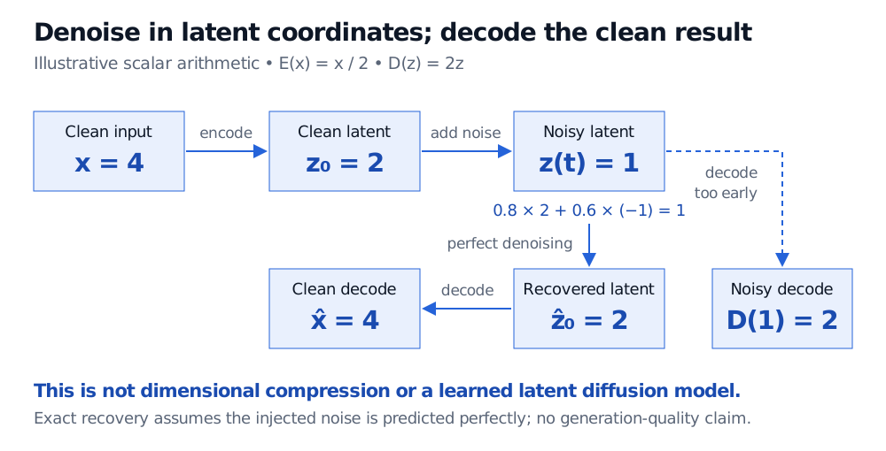
These maps are not dimensional compression, a learned autoencoder or a trained LDM. Both spaces have one coordinate. Take a dimensionless clean input x=4, so z0=2. With αˉt=0.64 and stipulated noise ϵ=−1,
zt=0.8(2)+0.6(−1)=1.
Decoding immediately gives D(1)=2, which is still corrupted. Assume a perfect noise predictor returns ϵ^=−1. Solving the forward equation gives
The decoder alone did not remove the noise. Nor does a real predictor receive the corruption draw at generation time. Exact recovery is stipulated here to expose the coordinate flow; this single clean estimate is not a complete reverse sampling trajectory.
Illustrative scalar flow: clean input 4 encodes to latent 2; artificial noise produces latent 1. Decoding it gives 2. Perfect denoising restores latent 2, then decoding gives 4. Both spaces remain one-dimensional.
Original dimensionless arithmetic, with a stipulated perfect predictor. Reversible scalar rescaling demonstrates where denoising occurs, not compression or learned generation quality.
What a financial application must preserve
Applying this architecture to a financial diffusion generator requires a financial representation and training objective. Image perceptual fidelity is not a test of return tails or liquidity shocks. As a practical inference, test the encoder–decoder reconstruction on held-out stress observations before assessing generated scenarios: a representation that erases a joint sell-off may hide a risk failure behind a small average reconstruction error.
Then assess generated data in original units, including tails, cross-asset dependence and the downstream risk calculation. Fit preprocessing and the representation within the historical training cutoff, and use only conditioning information available at the scenario date. Compression offers no automatic guarantee of these properties, and conditioning is not evidence of causal control.