How greedy selection, temperature and nucleus sampling turn next-token probabilities into text, and why decoding settings belong in a reproducible quant workflow.
Language model decoding
Language model decoding is the procedure that turns a model's next-token scores into an output sequence. For a quant using a large language model to label filings, decoding is part of the measurement procedure: the same document and model can yield different wording or labels under different selection rules.
This is generation-time selection, rather than training the model or converting token IDs back into readable characters. At each step the model supplies a conditional probability distribution given the prompt and generated prefix. The decoder selects a token, appends it, and repeats until a stopping condition is reached. Subsequent distributions depend on the token actually selected. Hugging Face's generation guide distinguishes greedy selection, sampling and beam search.
One context, several selection laws
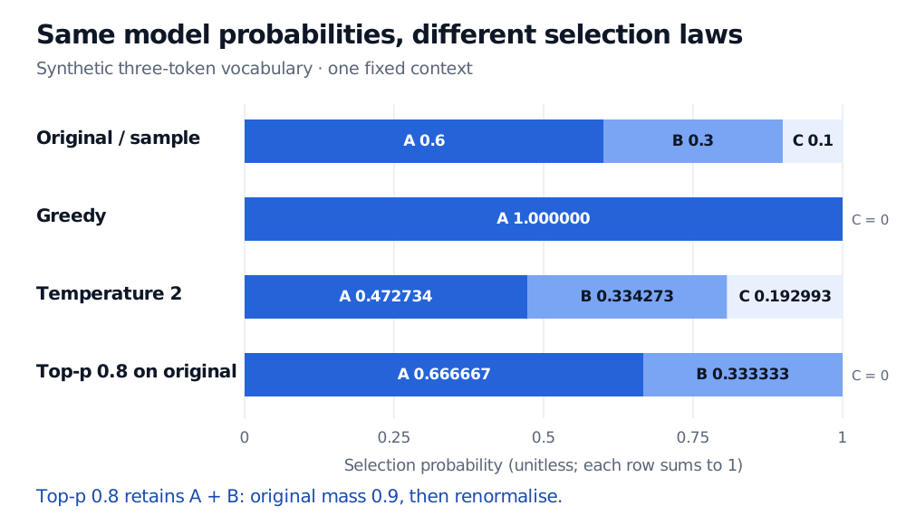
Suppose a synthetic vocabulary contains only tokens A, B and C, with next-token probabilities (0.6,0.3,0.1). These are invented probabilities for explaining the mechanism, not estimates from a financial document.
Greedy decoding chooses A, the largest-probability token. Its selection law is (1,0,0); the underlying model still assigned A probability 0.6. Unmodified sampling instead draws from (0.6,0.3,0.1), so B and C remain possible.
Temperature reshapes the probabilities before sampling. For logits zi, the softmax rule at temperature T>0 is
qi(T)=∑jexp(zj/T)exp(zi/T)=∑jpj1/Tpi1/T,
where pi is the original softmax probability. Thus T=1 leaves the law unchanged. In this example, T=2 normalises square roots:
A higher positive temperature flattens the law; a lower one sharpens it without changing token rankings. The formula does not permit division by zero. With a unique maximum, its limit as T→0+ concentrates on that maximum. An API's “temperature zero” behaviour is an implementation convention. With tied maxima, the mathematical limit shares mass among them, while a greedy implementation may break the tie deterministically.
Top-k sampling retains a fixed number of highest-probability tokens, then renormalises. Top-p sampling, also called nucleus sampling, instead retains the shortest probability-ranked prefix whose cumulative mass reaches a cutoff, then renormalises. These are the truncation rules in Holtzman et al.'s original nucleus-sampling paper, §§3.1–3.3.
Apply top-p with cutoff 0.8 to the original law. A alone has mass 0.6; A and B have mass 0.9, so both survive:
qnucleus=(0.6/0.9,0.3/0.9,0)=(2/3,1/3,0).
The cutoff is a cumulative mass target, not a minimum probability for each token. It also does not mean “80% probability of a correct answer.” Here we keep the token that reaches or crosses the cutoff, retain at least one candidate, and order equal-probability tokens by token ID. Other tie or minimum-candidate conventions can change boundary cases; none affect this untied example.
Synthetic next-token law: A 0.6, B 0.3, C 0.1. Greedy selects A. Temperature 2 gives 0.472734, 0.334273, 0.192993. Top-p 0.8 applied to the original law gives A two-thirds, B one-third, C zero.
Original synthetic example at one fixed context. Bars show the selection law, not the probability that the generated claim is true.
Order can change which tokens survive
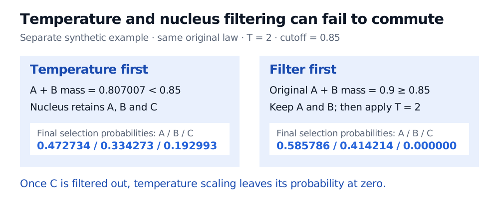
Use a separate cutoff of 0.85, still with T=2. Temperature first makes A and B sum to approximately 0.807007, below the cutoff: the nucleus includes C too. Filtering first on the original law keeps only A and B, whose original mass is 0.9. Applying temperature afterward gives approximately (0.585786,0.414214,0).
At cutoff 0.85, temperature 2 first keeps all three tokens because A plus B is 0.807007. Filtering the original law first keeps A and B with original mass 0.9; subsequent temperature 2 gives probabilities 0.585786 and 0.414214, with C zero.
Original ordering counterexample using a separate 0.85 cutoff. A filter can remove a token that later temperature scaling cannot restore.
At the earlier 0.8 cutoff, both orders happen to retain A and B and yield the same final law. Noncommutativity is possible, not inevitable. Record the actual processing order, constraints and defaults used by the serving system. The current GenerationConfig reference also distinguishes sampling, beam count, truncation, length penalties and stopping controls; supported settings depend on the implementation and model.
Token choice is not sequence search or verification
Beam search maintains several candidate prefixes and prunes them using sequence scores. For a fixed-length continuation, its unadjusted log-probability score sums conditional log-probabilities along that continuation. Length penalties and stopping rules can alter the ranking. A finite beam is an approximate search: choosing the best next token greedily need not find the best whole sequence, and even beam search need not find the global optimum. The three-token example above supplies no later conditional probabilities, so it cannot rank complete sequences.
Holtzman et al. found that probability-maximising search could produce repetitive open-ended text in their GPT-2 experiments. That historical result motivates examining the decoding objective; it does not establish a universally best decoder for every task. Increasing diversity also supplies no factuality guarantee.
For disclosure annotation, freeze the prompt, model version, decoding configuration and stop rules; retain actual responses. A seed alone does not identify all those conditions or guarantee identical outputs across serving changes. Then evaluate labels against checked human judgements. The LLM Annotation lesson develops that codebook and comparison; its preview is public and the full lesson requires membership. A stable wrong label remains wrong, and a fluent explanation still needs evidence from the correct issuer, period and document.
Sources
Ari Holtzman et al., The Curious Case of Neural Text Degeneration, ICLR 2020, §3 (sequence objective), §§3.1–3.3 (nucleus, top-k and temperature), and §§4.1, 5.3 (historical experimental setting and repetition).
Hugging Face Transformers, Generation strategies, “Basic decoding methods”: greedy search, sampling and beam search. Current documentation checked 1 November 2026.
Hugging Face Transformers, GenerationConfig, strategy, logit manipulation, length and stopping parameters. Current documentation checked 1 November 2026; no package-specific defaults are required for the calculations here.