Johnson-Lindenstrauss lemma and random projections: Definition & Examples

The Johnson-Lindenstrauss lemma says that a finite collection of high-dimensional points admits a much smaller Euclidean representation with approximately preserved pairwise distances. A suitably scaled random projection provides such a representation with high probability. For a quant researcher comparing many market feature vectors, this offers a way to compress the inputs to distance-based searches without first estimating a factor structure. The guarantee concerns geometry, not predictive performance. Dasgupta and Gupta give an elementary proof.

What is preserved?

Fix

n\ge 2

points

x_1,\ldots,x_n\in\mathbb{R}^{D}

, chosen independently of the random map, a tolerance

0<\epsilon<1

and a failure probability

0<\delta<1

. Here the tolerance applies to squared Euclidean distances:

(1-\epsilon)\lVert x_i-x_j\rVert_2^2 \le \lVert Ax_i-Ax_j\rVert_2^2 \le (1+\epsilon)\lVert x_i-x_j\rVert_2^2 \quad\text{for every }i,j.

One construction uses an $m\times D$ matrix with independent entries $A_{ab}\sim\mathcal{N}(0,1/m)$ . A sufficiently large target dimension of order

m=O\!\left(\epsilon^{-2}\log\frac{n}{\delta}\right)

makes the displayed inequalities hold simultaneously with probability at least

1-\delta

, over the draw of

A

. This is a sufficient scaling law, not a formula for the smallest workable dimension. The original dimension does not enter this order bound; if the sufficient dimension exceeds

D

, it offers no compression. Shalizi’s CMU notes state the Gaussian high-probability version; scikit-learn’s documentation confirms the entry variance.

The scaling matters: for a fixed vector $v$ , $\mathbb{E}[\lVert Av\rVert_2^2]=\lVert v\rVert_2^2$ . Correctness in expectation alone is insufficient. Concentration controls distortion for one difference vector; a union bound controls all $n(n-1)/2$ pairs. That is the source of the logarithmic dependence on dataset size.

Read the tolerance before checking a projection

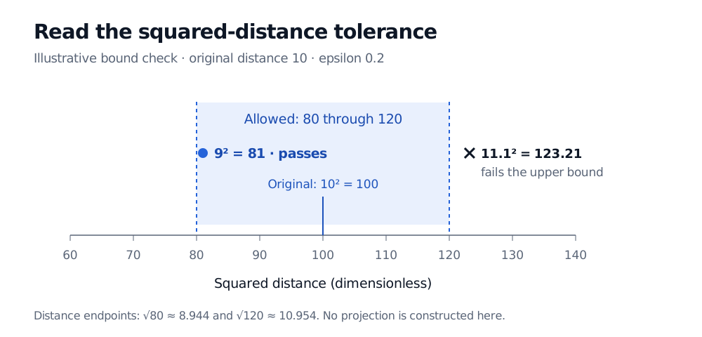
Suppose two dimensionless feature vectors are distance $10$ apart and $\epsilon=0.2$ . Their squared distance is $100$ , so the permitted projected squared distance is

80\le \lVert Ax_i-Ax_j\rVert_2^2\le120.

A projected distance of $9$ passes because $9^2=81$ . A distance of $11.1$ fails because $11.1^2=123.21$ . The distance interval itself is $[\sqrt{80},\sqrt{120}]$ , approximately $[8.944,10.954]$ —not $[8,12]$ . Some statements use an unsquared-distance tolerance; their epsilon must be interpreted accordingly.

Squared-distance tolerance for an original distance of 10 and epsilon 0.2. The permitted band is 80 to 120. A projected distance of 9 gives 81 and passes; 11.1 gives 123.21 and fails.

Illustrative bound check, not a constructed random projection. The shaded band applies to squared distances; its distance endpoints are about 8.944 and 10.954.

These hypothetical outputs only illustrate how to read the bound. They neither construct a projection nor establish that a chosen target dimension satisfies the theorem.

Compression without discovering factors

Unlike principal component analysis (PCA), the Gaussian map does not learn directions of greatest sample variance. It mixes coordinates randomly. Both perform dimensionality reduction, but preserving distances and extracting interpretable market factors are different objectives. The SelfMadeQuant lesson Principal Component Analysis and the SVD View develops the variance objective; its preview is public and the full lesson requires membership.

For a feature panel, decide what distance should mean before compressing it. If large numerical units dominate the original metric, preserving that metric preserves their dominance too. Approximate distances also allow close competitors to exchange nearest-neighbour rank; exact rankings require additional separation.

Finally, this is a guarantee for the specified finite set. The same matrix can transform new observations, but the event above does not certify all future or adaptively selected vectors. Indeed, when $m<D$ , a linear map has a nonzero null-space direction that it sends to zero. A claim to preserve every possible vector would contradict that fact. In financial research, monitor the geometry of new data and evaluate the downstream task separately; a distance guarantee cannot establish a trading signal.

Sources

Dasgupta and Gupta, An Elementary Proof of a Theorem of Johnson and Lindenstrauss (2003), Theorem 2.1 and its concentration/union-bound proof.
Cosma Shalizi, Dimension Reduction III (CMU, 2022), “Distance-preserving projections” through “Random projections are nearly distance-preserving with high probability”.
Scikit-learn, Random Projection, sections 8.6.1–8.6.2.

What is preserved?

Read the tolerance before checking a projection

Compression without discovering factors

Sources

Related terms

Dimensionality reduction

Euclidean norm