The bullwhip effect is the amplification of fluctuations in replenishment orders as demand information travels upstream from retailers to distributors and manufacturers. An inventory cycle is a period of stock building followed by a drawdown, or the reverse. When suppliers produce in response to a burst of orders and retailers later cut purchases to run down stock, factory activity can swing even if consumer purchases barely move. That distinction matters when using orders to forecast industrial output. Lee, Padmanabhan and Whang’s original study
Two weeks, the same mean and different swings
In a fictional two-week window, customers want 90 units in week 1 and 110 in week 2, and the retailer fills both weeks' demand. It places replenishment orders of 80 and 120 units at the end of each week. Both series average 100 units per week. Taking the two weeks as the entire equally weighted example, customer demand is 10 units away from its mean each week, giving a population variance of 100. Orders are 20 units away from their mean each week, giving a variance of 400.
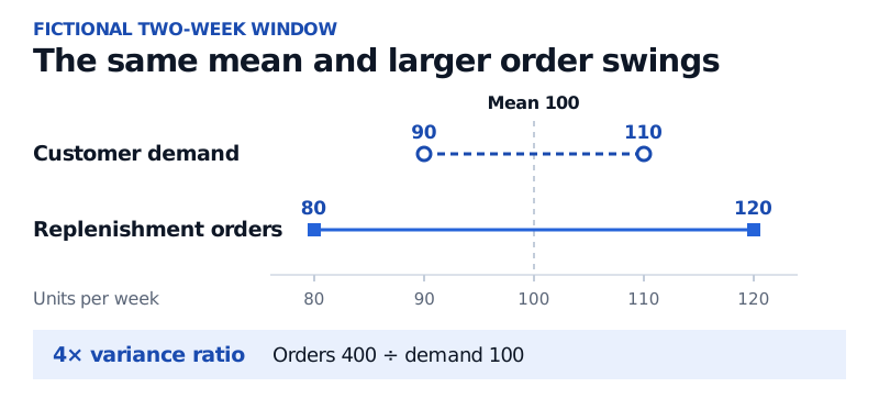
The two series have the same weekly mean. Doubling the distance from that mean quadruples the variance.
The fourfold ratio describes this fictional window. Two weeks give too little evidence to establish serial dependence, a recurring inventory cycle or a causal response to demand.
How a stock target amplifies orders
Suppose the retailer reviews stock after sales each week and tops up to a target inventory position. This position counts units on hand plus units already ordered and still due, less units owed to customers. When an outstanding order arrives, it moves from units due to units on hand. With all demand filled, no other adjustments and the previous week ending at its target position, the replenishment order equals units sold plus the change in the target, provided that quantity is positive.
One policy consistent with the example would lower the target by 10 units in week 1, so it orders 80 after selling 90. Raising the target by 10 in week 2 brings the order to 120 after 110 sales. Forecast revisions can change a target in this way. Batching purchases into full truckloads, buying ahead of an expiring discount, or ordering extra in anticipation of rationing can also widen order swings. Lee, Padmanabhan and Whang, Sections 3 and 4
On-hand stock follows a different balance. Ignoring returns and losses, the change in on-hand units equals receipts minus units sold. Placing an order raises the inventory position immediately, while on-hand stock rises only on receipt. If a large order arrives after sales cool, stock can build. The retailer may then cut future orders below sales to draw down stock, reducing its supplier’s order intake even while retail sales hold steady.
What the data can separate
Compare orders and demand for the same product and supply-chain link, using the same units, calendar frequency and sample window. A weekly ordering burst may disappear when the data are summed monthly. Check seasonality and trends before interpreting a ratio as short-run amplification. The ratio requires positive demand variance.
Point-of-sale data record what customers bought. During a stockout they can miss unmet demand, so a ratio using sales measures amplification relative to observed sales. Keep forecasts and their revisions separate from placed orders, and distinguish gross orders, cancellations and shipments. For example, the US Census Bureau’s manufacturing survey defines new orders net of cancellations and reports shipments and inventories separately. This aggregate series has a different scope and frequency from the retailer’s unit ledger. US Census Bureau, Manufacturers’ Shipments, Inventories, and Orders definitions
Why GDP can slow while inventories still rise
In the US national accounts, the change in private inventories is the inventory investment flow included in GDP. For the change in GDP between periods, what matters is how much that flow changes. In a fictional one-good economy at a fixed price, suppose final sales stay at 100 dollars per period and inventory investment slows from 20 dollars to 5 dollars. GDP falls from 120 dollars to 105 dollars as firms add less to stock. A retailer’s unit ledger explains how a stock adjustment can start. The national accounts measure the value of the change in physical inventories across the economy and exclude gains or losses from holding goods as prices change. BEA NIPA Handbook, Chapter 7
Sources
- Lee, H. L., Padmanabhan, V., and Whang, S. (1997). Information Distortion in a Supply Chain: The Bullwhip Effect. Management Science, 43(4), 546–558. Full text, Sections 3 and 4.
- US Census Bureau. Manufacturers’ Shipments, Inventories, and Orders definitions.
- US Bureau of Economic Analysis. NIPA Handbook, Chapter 7, Change in Private Inventories.