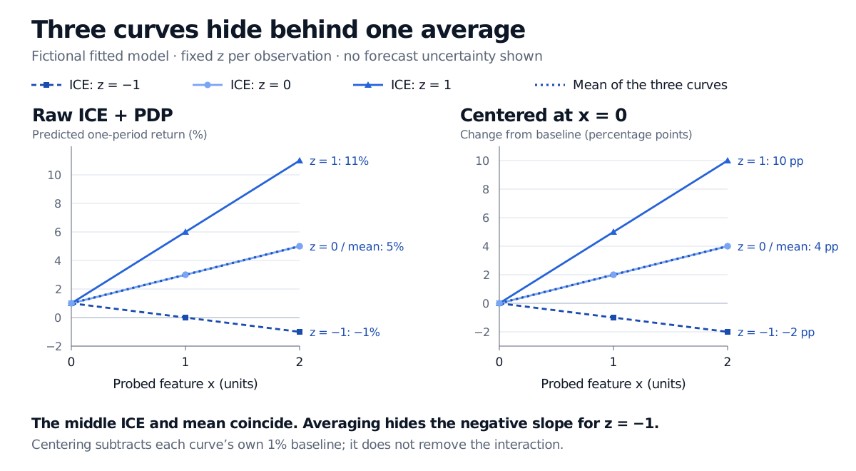
An ICE plot traces a fitted model’s prediction for each observation as one feature varies. See how opposite slopes disappear in a partial dependence average.
Individual conditional expectation plot
An individual conditional expectation (ICE) plot traces a fitted model’s prediction for each observation as one feature varies and that observation’s other inputs stay fixed. In quant model review, it can expose a forecast that rises with a signal in some market states but falls in others—behaviour an average curve can conceal.
For a fitted prediction function f^, a probed feature value u and observation i’s remaining inputs xi,−j, the curve is
ICEi(u)=f^(u,xi,−j).
The model stays fixed: it is evaluated repeatedly, without retraining. Despite the name, this is not a fresh estimate of the population conditional mean at each plotted point. The official scikit-learn guide describes one line per sample.
When the mean points in the wrong direction for one observation
Consider the fictional fitted function
f^(x,z)=0.01+0.02x+0.03xz,
predicting a decimal one-period return: 0.01 means 1%. Both inputs are dimensionless. Probe x at 0, 1 and 2 for three observations whose fixed z values are −1, 0 and 1. No observed future returns or prediction errors are supplied.
Fixed companion input
Prediction at x=0
At x=1
At x=2
z=−1
1%
0%
−1%
z=0
1%
3%
5%
z=1
1%
6%
11%
Equal-weight mean
1%
3%
5%
The slope is 0.02+0.03z: −1, +2 or +5 percentage points per unit of x. The xz term creates a feature interaction: the response to x depends on z.
A partial dependence plot formed by averaging these same three curves gives
PD(u)=31i=1∑3ICEi(u)=0.01+0.02u.
Its upward slope correctly describes this sample average. Reading it as “the prediction increases for every observation” is wrong: the z=−1 prediction decreases. The mean also depends on which observations are included and their weights.
Fictional ICE curves at x equal to 0, 1 and 2 predict 1%, 0% and −1% for z = −1; 1%, 3% and 5% for z = 0; and 1%, 6% and 11% for z = 1. The mean is 1%, 3% and 5%. Centering at x = 0 gives endpoint changes of −2, 4 and 10 percentage points.
Original fictional model probe. Each curve holds z fixed. The mean coincides with the z = 0 curve; centering changes levels and units, while preserving slopes.
Centering compares changes from a common feature value
Centered ICE subtracts each curve’s own prediction at a chosen reference u0:
cICEi(u)=ICEi(u)−ICEi(u0).
Goldstein and co-authors, §3.2, introduce this to remove differences in baseline levels. Here, choosing u0=0 subtracts 1% from every curve. At x=2, the centered values are −2, +4 and +10 percentage points; their mean is +4 points. These are changes in predicted return, not percentage growth rates of the forecasts.
The differing slopes remain. If a model is additive in the probed feature, f^(x,z)=g(x)+h(z), centering makes its curves coincide. Divergence therefore helps diagnose interactions in the fitted function over the inspected inputs; it does not establish an economic mechanism.
INTERACTIVE EXPLORER
ICE curves and average dependence
Vary one input of a fixed interaction model while holding each context fixed.
Check whether the probe describes plausible inputs
Holding other features fixed can create unsupported combinations when inputs are correlated. Varying a valuation ratio while freezing its component prices, for example, can break a feature-construction identity. A point can lie inside every individual feature’s range yet outside the observed joint support. The scikit-learn guide warns about this artificial-input problem.
Inspect joint support and mark observed feature values; treat unsupported regions as extrapolation. The original ICE paper’s §4.3 demonstrates this diagnostic.
An ICE curve is a feature probe, not a causal intervention. It shows what a fixed model returns for substituted inputs, not what trading or changing an economic variable would cause. Zhao and Hastie, §§1–3, explain why causal interpretation requires additional causal assumptions. The spread between curves reflects differences in their fixed inputs; it is not a confidence band and does not represent uncertainty about the fitted model or future returns.
For the separate question of auditing a ranking of model inputs, see Feature importance (public preview; full lesson requires membership).
Zhao and Hastie, Causal Interpretations of Black-Box Models: §§1–3 distinguish fitted-function behaviour, predictive importance and causal effects, and state the additional causal-structure requirements. Author manuscript dated 3 October 2018.