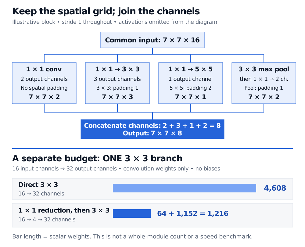
How Inception joins parallel convolution scales, keeps branch shapes compatible and reduces a single branch from 4,608 to 1,216 weights with a channel bottleneck.
Inception network and multiscale convolution
An Inception network is a convolutional neural network built around blocks that process the same input through parallel branches at different spatial scales, then concatenate their features along the channel axis. For a quant experimenting with grid-shaped data, such as a volatility surface, the attraction is the ability to combine local detail and wider context without committing every feature to one kernel size. That architectural motivation does not establish forecasting value.
Several views of the same input
The original Inception module combines a 1 × 1 convolution, a 3 × 3 path, a 5 × 5 path and a pooling path. The larger-kernel paths use 1 × 1 channel reductions first; the pooling path uses a 1 × 1 projection afterward. GoogLeNet is the particular full network described in the original paper, rather than another name for every later Inception design. See Szegedy et al., §§4–5.
A 1 × 1 convolution mixes channels at each location. It does not gather neighbouring locations itself. The wider kernels gather different spatial neighbourhoods; pooling supplies an alternative local aggregation. These paths are trained together, rather than fitted as independent models whose final predictions are averaged.
Consider an illustrative block, not a reproduction of a GoogLeNet layer. Write tensor shapes as height × width × channels and omit the batch axis. All branches receive a 7 × 7 × 16 input:
Branch
Final branch output
Shape convention
1 × 1 convolution
7 × 7 × 2
Stride 1; no spatial padding
1 × 1 reduction → 3 × 3 convolution
7 × 7 × 3
Stride 1; one cell of padding around the 3 × 3 input
1 × 1 reduction → 5 × 5 convolution
7 × 7 × 1
Stride 1; two cells of padding around the 5 × 5 input
3 × 3 max pooling → 1 × 1 projection
7 × 7 × 2
Pool stride 1 and one cell of border padding
The output is 7 × 7 × 8, because channel counts add: 2+3+1+2=8. Concatenation keeps the branch features as distinct channels; it does not add their values element by element, as a residual connection would.
The common spatial shape is essential. A stride-2 pooling branch would produce a different grid and could not be concatenated here without an explicit alignment operation. Padding must also use an appropriate border convention: for max pooling, padded entries must not spuriously dominate negative activations. The D2L Inception implementation illustrates stride-1 pooling and compatible branch padding.
Illustrative four-branch Inception block preserves a 7 by 7 grid and concatenates 2, 3, 1 and 2 channels into 8. A separate single 3 by 3 branch with 16 input and 32 output channels uses 4,608 weights directly, or 64 plus 1,152 equals 1,216 with a four-channel bottleneck; biases excluded.
Original illustrative architecture and separate branch budget. Shapes use height × width × channels; the lower comparison does not count the four-branch block above.
Why reduce channels before widening the view?
Now isolate one different branch with 16 input channels and 32 output channels. Exclude biases. A conventional dense 3 × 3 convolution has
3⋅3⋅16⋅32=4,608
scalar filter weights. First reducing 16 channels to four with a 1 × 1 convolution, then applying a 3 × 3 convolution from four to 32 channels, gives
(1⋅1⋅16⋅4)+(3⋅3⋅4⋅32)=64+1,152=1,216.
The spatial convolution now reads four channels per location instead of 16. These are single-branch weight counts, not total module parameters, activation-memory measurements or latency benchmarks. A narrow bottleneck also constrains the representation: fewer weights do not guarantee equal predictive quality. In the original architecture, reductions include rectified linear activations; the two-stage path is not generally an algebraically identical replacement for an arbitrary direct convolution. Original design, §4.
Original blocks, later variants and financial grids
Later Inception work explores replacing larger filters with sequences of smaller convolutions and factorising spatial operations into asymmetric kernels, such as 1 × n followed by n × 1. These are later design developments; they should not be silently inserted into a diagram labelled as the original module. Nor does matching a nominal receptive field make two nonlinear architectures identical. Rethinking Inception, §§3.1–3.2.
On a volatility surface, a wider patch could gather information across nearby maturities and strikes. This is a proposed use of the architecture, not an empirical result here. Grid spacing matters: neighbouring cells need a stable interpretation across observations. On a time-indexed input, centred convolution or pooling may consume later observations; a forecasting design must restrict every branch to information available at its prediction time. Different kernel sizes alone do not enforce that restriction.