Successive halving reallocates training to surviving trials; Hyperband varies how aggressively it starts. Track total budgets, resumed compute and chronological validation.
Successive halving and Hyperband
Successive halving is a resource-allocation procedure for hyperparameter tuning: evaluate candidates cheaply, discard the weaker ones and give survivors more training. Hyperband runs several such searches, called brackets, with different starting budgets and candidate counts. For a financial forecasting model, this can save training effort while exploring more settings; it does not make the selected forecast independently validated.
One bracket, two ways to count its cost
Suppose a researcher compares nine configurations of the same neural-network training task. One resource unit is one epoch over a fixed, eligible training dataset. All candidates use the same validation dates and loss; lower loss is better. The following is a hypothetical allocation schedule, with no fitted performance results.
Use an elimination factor of η=3: retain the best third at each decision.
Stage
Configurations trained
Total epochs per configuration
Extra epochs if resumed
1
9
1
1
2
3
3
2
3
1
9
6
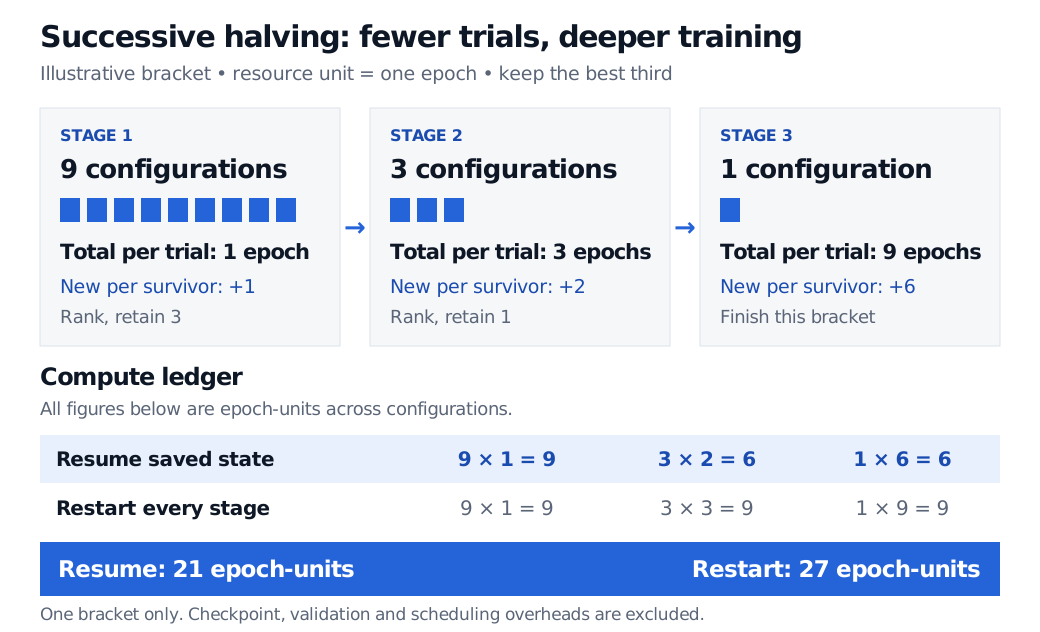
After stage 1, stop six candidates. Continue three to three total epochs, then continue one to nine total epochs. The final stage completes the surviving trial; it makes no new comparison with the eight discarded trials.
If saved training state can be resumed faithfully, new training work is
9×1+3×(3−1)+1×(9−3)=21
epoch-units across configurations. Another way to audit this is by final lifetime: six discarded trials receive one epoch each, two receive three each, and one receives nine, totalling 21.
If every stage instead trains its candidates from scratch to that stage's total budget, the work is
9×1+3×3+1×9=27.
Both calculations describe the same allocation targets. They describe different execution policies. Resumption needs compatible saved weights, optimiser state and training schedule; restarting merely from saved weights need not reproduce uninterrupted training. Validation, checkpointing, loading and scheduling costs are excluded, and an epoch can cost more for a larger model. These are training-work counts, not measured wall-clock savings.
One illustrative bracket trains 9 configurations to 1 epoch, 3 survivors to 3 total epochs and 1 survivor to 9 total epochs. Resuming adds 9, 6 and 6 epoch-units for 21 total; restarting uses 9 at each stage for 27 total.
Original hypothetical allocation diagram. Epoch budgets are totals per configuration, not extra epochs at each stage. The compute comparison excludes overhead and assumes resumable training.
Hyperband varies the starting bet
A large starting population explores widely but gives each candidate little evidence before elimination. A smaller population can train longer before its first comparison. Li and colleagues' Hyperband algorithm, §3, spreads resources across both kinds of bracket. Its least aggressive bracket evaluates sampled configurations at the maximum resource without early elimination. The original method samples configurations randomly; the allocation rule is distinct from a model that proposes settings using previous results.
The nine-to-three-to-one schedule above is one successive-halving bracket, not a complete Hyperband run. Other brackets consume additional resources.
Early rank can mislead. A slowly improving configuration may be discarded before it beats a fast starter. Hyperband's conservative brackets reduce dependence on one aggressive schedule, but do not guarantee that a particular search finds the best full-budget candidate. The official scikit-learn guide likewise stresses whether small resource allocations can distinguish candidates. Its halving searches implement successive halving; one such search is not automatically all of Hyperband's brackets.
Training budget is not an information boundary
For historical financial forecasts, keep the resource schedule inside a valid chronological experiment. Prefer varying training effort on the same eligible history when the aim is to compare optimisation progress. Reducing the data budget changes the information and possibly the market regimes represented, not just the computation.
At each simulated fit time, training labels must already be available and learned preprocessing must use permitted data. Rank candidates on subsequent development validation observations, then preserve a later test set for assessment of the frozen selection procedure. Rolling-origin evaluation uses preceding observations to forecast later ones, as explained in Forecasting: Principles and Practice. A cheaper search does not prevent look-ahead bias or overfitting repeated validation comparisons.