Hierarchical agglomerative clustering: Definition & Examples

Hierarchical agglomerative clustering builds nested groups by starting with each observation alone and repeatedly merging the closest pair of clusters under a chosen linkage rule. In quantitative research, this can reveal several resolutions of asset peer groups rather than forcing one partition at the outset. The resulting tree describes the geometry of the supplied data; it does not establish permanent economic sectors.

This is a form of unsupervised learning. Unlike the flat k-means example in clustering, it records a sequence of nested partitions. Agglomeration proceeds from individual observations upwards; divisive hierarchical methods instead split groups downwards. The scikit-learn guide distinguishes these directions.

Two choices hidden inside “closest”

First choose a distance between observations. Then choose how distances between whole clusters are defined. For clusters $A$ and $B$ , with observation distance $d(i,j)$ , three common rules are:

Linkage	Distance between clusters	What drives the next merge
Single	Smallest distance across the two groups	Their closest pair of observations
Complete	Largest distance across the two groups	Their farthest pair of observations
Average	Mean of all cross-group pair distances	Every cross-group pair, equally weighted

Average linkage here means UPGMA: average over observation pairs, not an unweighted average over previous cluster summaries. At each step, merge the cluster pair with the smallest value of the selected criterion, then recalculate distances involving the new cluster. Existing merges are retained. SciPy's linkage reference gives these definitions.

Single linkage can join extended chains through nearby neighbours even when their endpoints are far apart. Complete linkage penalises that farthest separation; average linkage lies between the minimum and maximum cross-pair distances for a given pair of clusters. None is universally the correct geometry.

Three observations, three final heights

Take an original synthetic one-dimensional dataset,

0,2,5

, in arbitrary feature units, using Euclidean distance. The pair distances are

2

3

and

5

. Single, complete and average linkage all first merge observations

0

and

2

at height

2

The remaining comparison is between $A=\{0,2\}$ and $B=\{5\}$ . Its two cross-group distances are $5$ and $3$ :

\begin{aligned} D_{\mathrm{single}}(A,B)&=\min(5,3)=3,\\ D_{\mathrm{complete}}(A,B)&=\max(5,3)=5,\\ D_{\mathrm{average}}(A,B)&=\frac{5+3}{2}=4. \end{aligned}

The memberships merge in the same order in this tiny dataset, but the second merge height differs. In larger datasets the choice can change the merge order too.

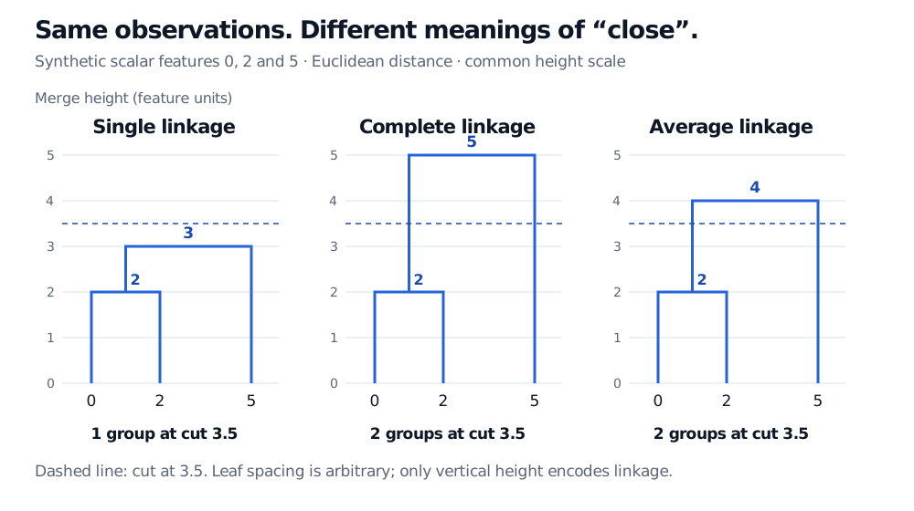
Synthetic scalar observations 0, 2 and 5 merge first at height 2. Final heights are 3 for single linkage, 5 for complete linkage and 4 for average linkage. A cut at 3.5 gives one group for single linkage and two for the others; leaf spacing is arbitrary.

Original synthetic example, with Euclidean distances in feature units. All three panels use the same height scale. The dashed cut is a chosen resolution, not a statistically established boundary.

A dendrogram displays that merge history. Read vertical heights as the selected linkage values, as described in SciPy's dendrogram reference. Horizontal leaf spacing is a layout choice, not the distance between observations.

For the three linkage rules shown, cut horizontally at height $3.5$ , retaining merges below the cut. Single linkage has already joined all three observations, giving one group. Complete and average linkage still give two groups: $\{0,2\}$ and $\{5\}$ . Thus a height threshold needs its linkage convention. Alternatively, choose a desired cluster count and cut the tree accordingly; specify tie handling when merges share a height.

Ward linkage answers a different question: it chooses the merge with the smallest increase in total within-cluster squared error. Its reported heights need their implementation's convention, and Ward requires Euclidean geometry. Do not feed it an arbitrary dissimilarity matrix merely because other linkage rules accept one. The SciPy notes state this restriction.

Before interpreting asset groups

Feature scaling is part of the model. Combining volatility and turnover without an explicit scaling choice can make one coordinate dominate Euclidean distances. Even uniformly multiplying every scalar value here by ten multiplies all three trees' heights by ten while preserving their merge order. A fixed numerical cut would then mean something different. Rescaling individual coordinates in a multivariate dataset can also change the tree itself.

For financial use, state the asset universe, observation window, features, scaling, distance, linkage and cut. Compare nearby windows and reasonable modelling alternatives before interpreting a branch as an economic peer group. A dendrogram is neither a significance test nor evidence that a historical grouping will remain stable.

If the groups enter a backtest, respect the decision-time information boundary: fitting the tree or feature scaling on later observations introduces look-ahead bias. Also specify how a newly arriving observation receives a group; an agglomerative tree does not automatically supply a prediction rule for unseen rows. The scikit-learn clustering guide identifies this transductive limitation, while its leakage guidance explains the training-data boundary.

For a useful comparison, the k-Means Clustering lesson develops centroid assignments and their squared-distance objective. The full lesson requires membership, with a public preview.

Sources

SciPy: linkage, linkage definitions, merge representation, tie warning and Euclidean restrictions.
SciPy: dendrogram, interpreting branches and merge distances.
scikit-learn: Clustering, §2.3.6 on hierarchical methods, linkage choices and metrics; §2.3.1 on transductive methods.
scikit-learn: Common pitfalls — data leakage, §12.2 on fitting transformations using training information only.

Two choices hidden inside “closest”

Three observations, three final heights

Before interpreting asset groups

Sources

Related terms

Clustering

Look-ahead bias

Unsupervised learning