Harmonic and geometric mean: Definition & Examples

The harmonic mean averages reciprocals and then takes the reciprocal; the geometric mean averages logarithms and then exponentiates. They answer different financial questions: the harmonic mean gives average purchase cost when equal cash amounts buy at different positive prices, while the geometric mean gives the constant growth factor that reproduces compounded returns. Choose the quantity being preserved before choosing the mean.

For $n\ge1$ strictly positive observations $x_1,\ldots,x_n$ , the three familiar means are

A=\frac{1}{n}\sum_{i=1}^n x_i, \qquad G=\left(\prod_{i=1}^n x_i\right)^{1/n} =\exp\left(\frac{1}{n}\sum_{i=1}^n\log x_i\right), \qquad H=\frac{n}{\sum_{i=1}^n 1/x_i}.

Here

A

is the ordinary arithmetic sample mean. These definitions use equal weights; the positive domain makes both the reciprocals and real logarithms well defined. NIST's treatment of means gives the definitions and their weighted generalisation.

A zero average percentage return can still lose money

Consider a fictional investment earning +20% and then −20% over two equal-length periods. Start with a wealth index of 100, retain all income and assume no external cash flows, fees or taxes. Its gross return factors are 1.20 and 0.80:

100\times1.20\times0.80=96.

The arithmetic mean simple return is zero, but compounding produces a 4% total loss. The constant per-period simple return

g

must solve

100(1+g)^2=96

, so

1+g=\sqrt{1.20\times0.80}\approx0.979795897, \qquad g\approx-2.0204103\%.

The geometric mean is taken over gross factors $1+r_i$ , followed by subtracting one. Taking a geometric mean directly over signed percentage returns does not reproduce this wealth calculation. The return calculations in Eric Zivot's university notes distinguish products of gross returns from sums of simple returns.

For the same two gross factors,

A=1

G\approx0.979795897

and

H=0.96

. That harmonic mean happens to equal the two-period product in this example, but it is not the equivalent per-period growth factor: repeating 0.96 twice ends at 92.16, rather than 96.

With

n

equal periods, the equivalent compound return is

G(1+r_1,\ldots,1+r_n)-1

. When each period is one year, this is the observed compound annual growth rate. Unequal observation intervals require an explicit time unit: the annual equivalent uses the product of the factors raised to the reciprocal of total elapsed years, rather than automatically taking an

n

th root.

Equal cash purchases ask a different question

Buy the same fictional share at two prices, USD 100 and USD 200 per share. Ignore fees and allow fractional shares. Spend USD 100 at each purchase:

Purchase	Price per share	Cash spent	Shares acquired
First	USD 100	USD 100	1
Second	USD 200	USD 100	0.5
Total	—	USD 200	1.5

The average cost per share is total cash divided by total shares:

\frac{200}{1.5} =\frac{2}{1/100+1/200} =H(100,200) \approx\text{USD }133.33.

The lower-price purchase buys more shares, which is why simply averaging the two prices gives the wrong cost for this ledger. Buying one share at each price instead costs USD 300 for two shares, making the arithmetic average USD 150 correct for that different exposure. Neither figure is a forecast of the next price or evidence that either purchase policy will outperform.

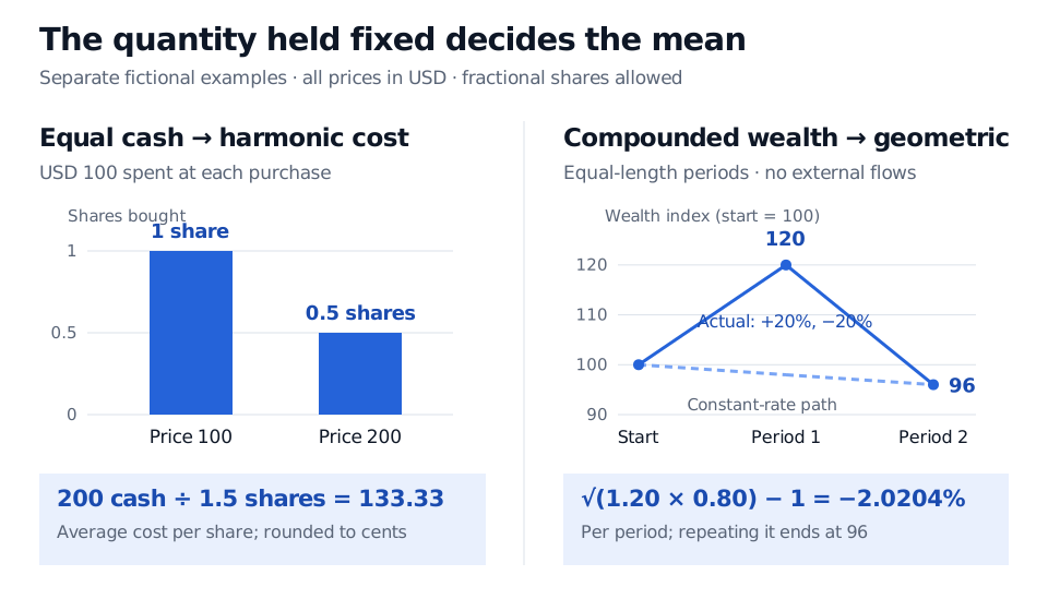
Separate fictional examples: equal USD 100 purchases at prices 100 and 200 buy 1 and 0.5 shares, giving average cost USD 133.33 per share. A wealth index earning plus 20% then minus 20% follows 100, 120, 96; constant geometric growth of minus 2.0204% per period reaches the same 96.

Original fictional examples. Left: equal cash fixes the numerator of price and varies shares bought. Right: solid blue shows observed period-end wealth; dashed blue shows the equivalent constant-rate path. Connecting lines do not describe within-period trading.

Weights and the positive domain are part of the definition

For nonnegative weights $w_i$ summing to one, retain strictly positive $x_i$ wherever $w_i>0$ . Omit zero-weight observations. Then

A_w=\sum_i w_i x_i, \qquad G_w=\exp\left(\sum_i w_i\log x_i\right), \qquad H_w=\left(\sum_i\frac{w_i}{x_i}\right)^{-1}.

In a purchase ledger with positive prices $P_i$ , positive cash amounts $C_i$ and quantities $q_i=C_i/P_i$ , the same average cost can be expressed two ways:

\frac{\sum_i C_i}{\sum_i q_i} =\left(\sum_i\frac{C_i}{\sum_j C_j}\frac{1}{P_i}\right)^{-1} =\sum_i\frac{q_i}{\sum_j q_j}P_i.

It is a cash-weighted harmonic mean of prices and a share-weighted arithmetic mean of prices. The weights change with the representation. “Use a harmonic mean for ratios” is incomplete advice: first identify the numerator, denominator and exposure being aggregated.

For positive observations and the same weights, the arithmetic–geometric–harmonic ordering is

H_w\le G_w\le A_w.

Equality throughout holds precisely when all observations with positive weight are equal. The concavity of the logarithm gives

\sum_i w_i\log x_i\le\log A_w

through Jensen's inequality, hence

G_w\le A_w

. Applying the same argument to

1/x_i

gives

H_w\le G_w

. Boyd and Vandenberghe develop this Jensen and AM–GM connection, §§3.1.8–3.1.9.

A zero observation makes the reciprocal and finite-log formulas unusable as written. For nonnegative data, a zero can be handled through an explicitly stated limiting convention for $G$ or $H$ ; it must not be silently dropped. In a no-flow investment, a zero gross factor means complete loss, with no finite log return. Negative observations generally invalidate this real-log framework and the stated ordering, even if a particular product has a real root. Signed rates, short positions and negative wealth therefore need separately defined accounting rather than these formulas applied mechanically.

Finally, the ordering compares summaries of a specified dataset. It does not establish that the lowest mean is the most prudent forecast or that the highest is the correct expected return. Backtest Evaluation connects linked growth to cash-flow treatment, costs and risk. Its preview is public; the full lesson requires membership.

Practice: identify the weights

A fictional investor spends USD 120 at USD 40 per share and USD 240 at USD 80 per share, with no fees and fractional shares allowed. What is the average cost per share, and why does the unweighted harmonic mean fail?

Answer. Each purchase buys three shares, so the average cost is

360/6=\text{USD }60

. The cash weights are

1/3

and

2/3

, giving the weighted harmonic mean

[(1/3)/40+(2/3)/80]^{-1}=60

. The unweighted harmonic mean is approximately USD 53.33; it would describe equal cash amounts at the two prices. Here the arithmetic mean of the two prices works because the share quantities are equal.

Sources

NIST Digital Library of Mathematical Functions, §1.2(iv), “Means”: equations 1.2.17–1.2.26 define arithmetic, geometric, harmonic and weighted power means, including positive-input conditions.
Eric Zivot, Return Calculations, updated 24 June 2014: §1.2.1, especially equation 1.9 for multiperiod gross returns; pp. 14–15 for equivalent annual rates; §1.2.2 for log returns. The examples here are original fictional ledgers and paths.
Stephen Boyd and Lieven Vandenberghe, Convex Optimization (2004), §§3.1.8–3.1.9, pp. 77–78: Jensen's inequality and the arithmetic–geometric mean inequality through the convexity of negative logarithms.

A zero average percentage return can still lose money

Equal cash purchases ask a different question

Weights and the positive domain are part of the definition

Practice: identify the weights

Sources

Related terms

Compound annual growth rate

Compounding