A fully convolutional network (FCN) is a convolutional neural network that processes a spatial or temporal grid without flattening it into a fixed-width vector for a fully connected layer. Shared filters let the same learned model process different grid sizes, subject to its kernel, stride and padding constraints. For a quant working with sequential observations, this separates two decisions: how to extract local patterns, and whether to retain their positions or summarise the whole window.
"Fully convolutional" does not mean every operation is a convolution: activations, pooling and upsampling can participate. Its grid of predictions can remain spatially indexed; optional global pooling is a subsequent readout. Long, Shelhamer and Darrell, §3.
A shrinking grid is still a grid
Consider a toy 1D network, not a reproduction of the original image-segmentation architecture. Take eight sequential input positions and apply two convolutions, each with kernel width three, stride one, dilation one and valid padding, meaning no padding. Ignore the batch and channel dimensions when counting positions.
For one such layer, the output length is
The first layer has six complete windows; the second has four. Thus . Each final position depends on five original positions: the first covers input positions one through five, and the last covers four through eight. These are overlapping local views, not four independent samples. The padding and shape conventions match the official Keras Conv1D documentation.
The filters can also slide across a longer input without acquiring new weights. For example, ten input positions would produce lengths eight and six under the same rules. Variable input size does not imply unchanged output size, nor does it guarantee that a model trained on short windows will generalise to much longer ones.
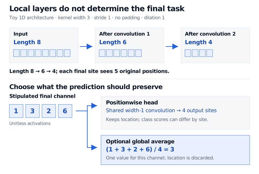
Original illustrative architecture: local feature extraction and the final readout make different choices about position.
Four predictions or one summary?
A positionwise head applies the same channel-mixing rule at each remaining location. A width-one convolution can produce class scores at each of the four output sites without mixing those sites together. Here “dense prediction” means predicting across locations; it does not mean attaching a fully connected dense layer.
For a different task, suppose one final channel has stipulated unitless activations . These values are supplied for the readout example, not calculated from unspecified input values or filters. Optional global average pooling gives
This returns one value for that channel, as described by the Keras global-average-pooling documentation. It is a feature summary, not automatically a probability or forecast. Averaging would also return three if those four activations were reordered: their location has been discarded. If the target is a label at each position, that summary cannot replace a positionwise head. Global average pooling is optional, not a defining requirement of an FCN.
Why the name is associated with segmentation
Long, Shelhamer and Darrell's 2015 work adapted image classifiers into networks producing spatial class-score maps. Fully connected layers were reinterpreted as convolutions; upsampling connected coarse predictions back to pixels. Their skip architecture combined coarse semantic information with finer features. That is a two-dimensional dense-prediction application of the FCN idea, rather than the global-average readout above. Upsampling restores output resolution, not a guarantee that all discarded detail has been recovered. Original paper, §§3.1, 3.3 and 4.1–4.2.
For a worked continuation, Dense Prediction: Segmentation Heads and Encoder–Decoder Intuition explains decoder resolution and skip connections. The preview is public; the full lesson requires membership.
For financial sequences, keep causality separate from architecture. A valid convolution looking at positions one through five is available only after position five has arrived; attaching its output to position one would introduce look-ahead bias. A temporal convolutional network adds sequence-specific design choices; the FCN label alone does not promise causal predictions. Likewise, a global summary of a completed window can serve an end-of-window decision but cannot retroactively become an earlier signal.