FT-Transformer is a neural architecture that turns each column value in a tabular observation into a feature token, then processes those tokens with a Transformer model. FT stands for Feature Tokenizer. For a quant researcher, it offers a way to model interactions between fields such as leverage, liquidity and sector in the same issuer snapshot. Its tokens represent features within a row, rather than successive dates.
Gorishniy and colleagues introduced the model in their 2021 paper Revisiting Deep Learning Models for Tabular Data. The model embeds numerical and categorical features, adds a learned CLS summary token, and predicts from CLS after Transformer layers. Those layers combine self-attention and feed-forward transformations with residual connections. CLS can support regression as well as classification; its name does not restrict the task.
A column needs its own identity
For numerical feature , the tokenizer uses
Here is a scalar, while the learned weight and bias are vectors of the common token width . Each feature has its own parameters. Two equal scalar values in different columns need not produce equal tokens. A leverage score of two and a liquidity score of two do not mean the same thing.
A categorical feature instead uses a categorical embedding: its category selects a vector from that feature's lookup table, with a feature-specific bias added. An integer category code is an address for a lookup; it is not a quantity to multiply as though sector four were twice sector two. These details are visible in the authors’ Tokenizer implementation.
Consider a fictional issuer row with a numerical leverage score of and sector “utilities”. Choose token width and stipulate the numerical column's parameters as and . Then
These are illustrative parameters, not estimates from financial data. The result is a representation, not a return forecast or a probability. The utilities token comes from a separate sector lookup; the leverage weights are not reused for it.
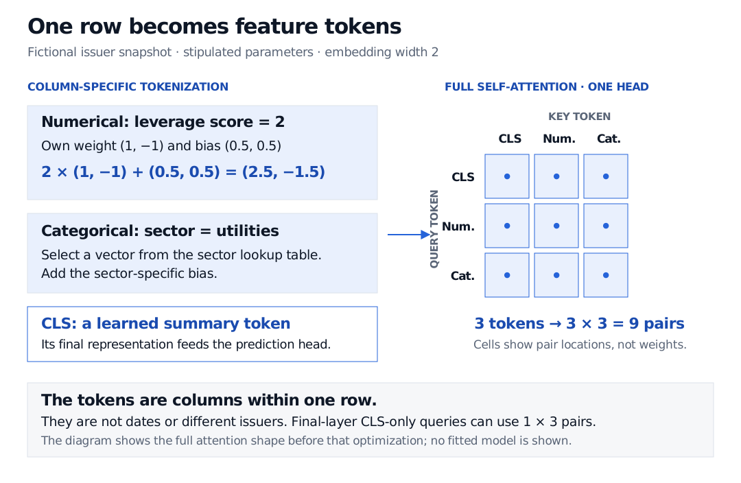
Original schematic with stipulated parameters. Attention operates across columns of one observation; the final-layer CLS-only optimization has three query–key pairs per head.
Count columns, not dates
The two feature tokens plus CLS give three tokens. In full self-attention, each of three queries can compare with three keys, so each head has a attention map: nine entries. This counts locations, not the values of the weights. The tokenizer alone does not specify those weights; query and key projections are still needed.
There is an implementation detail behind that count: in their final Transformer layer, the authors compute only the CLS query, because only its output is needed for prediction. Without key compression, that last attention map is , rather than the full map illustrated above. See Transformer.forward in the original code.
A row may contain lagged returns as separate columns, but tokenizing them does not automatically create a temporal forecasting model. The row construction must still encode which observations were available at prediction time. Full attention also becomes expensive as the feature count grows: the number of query–key pairs grows quadratically.
What would justify using it?
The original study found strong FT-Transformer performance across its benchmarks, while also finding strong simple neural baselines and no universal winner between deep models and gradient-boosted trees. That benchmark result does not establish superiority for a financial panel.
For an issuer-date prediction task, compare it with tuned tree models and simple neural models using the same target, features and held-out dates. Fit scaling, imputation and category handling on training data; choose settings on validation data; reserve a later test period for the final comparison. A random row split can place future observations in training, creating look-ahead bias for a forecasting claim. Report the prediction metric alongside training cost and inference latency.
Before tokenization, Tabular and Time-Indexed Data develops alignment and missing-value discipline for financial panels. The full lesson requires membership, with a public preview. Clean alignment is a necessary input check; it does not itself establish point-in-time availability.
Sources
- Gorishniy, Y., Rubachev, I., Khrulkov, V. and Babenko, A. (2021), Revisiting Deep Learning Models for Tabular Data, NeurIPS. Read §§3.3, 4.4–4.5 and Appendix E.1 for tokenization, architecture, comparisons and limitations. Linked HTML is the authors’ revised arXiv version dated 26 October 2023.
- Authors’ original FT-Transformer implementation, specifically
Tokenizer,MultiheadAttentionandTransformer.forward. The last-layer CLS-query optimization explains why a computed final attention map can be smaller than the full feature-to-feature map.