A centred partial-dependence measure of model interaction strength, with an exact four-point example and the limits of its variance-share interpretation.
Friedman H-statistic
The Friedman H-statistic measures departure from additive feature effects in a fitted prediction model, using centred partial-dependence functions. For a quant inspecting a return forecast, it helps distinguish “momentum and liquidity each contribute” from “momentum's contribution depends on liquidity”. It measures a model's feature interaction, rather than establishing an economic cause.
Subtract the main effects, then measure what remains
Fix a fitted scalar prediction function f^ and reference observations x(1),…,x(n). For a feature subset A, the empirical partial dependence function averages predictions after substituting the chosen feature values:
PA(zA)=n1r=1∑nf^(zA,x−A(r)).
Here −A means the remaining features. Centre each function over the evaluation observations, using the same weights throughout:
FA(zA)=PA(zA)−n1i=1∑nPA(xA(i)).
For two features j,k, subtract the two main effects from their joint effect:
The denominator must be positive. This is the pairwise normalisation in Friedman and Popescu's original paper, equation (44). The separate Hj statistic compares one feature with all remaining features together and normalises by centred full-model predictions, as in equation (45). Pairwise and overall scores answer different questions.
Four predictions make the calculation visible
Consider the fictional score model
f^(x1,x2)=x1+x2+x1x2,
where X1,X2 are independent, each taking −1 and +1 with equal probability. All four combinations therefore have weight 1/4. The score has arbitrary units; it is not a fitted return or default probability.
Averaging over the other feature gives F1(x1)=x1 and F2(x2)=x2. The joint function already has mean zero, so F12=f^. The residual is x1x2:
x1
x2
Joint score F12
Sum of mains F1+F2
Residual
−1
−1
−1
−2
+1
−1
+1
−1
0
−1
+1
−1
−1
0
−1
+1
+1
3
2
+1
Thus the mean squared joint score is (1+1+1+9)/4=3 and the mean squared residual is 1. Dividing sums or means gives the same ratio:
H122=31≈0.3333,H12=31≈0.57735.
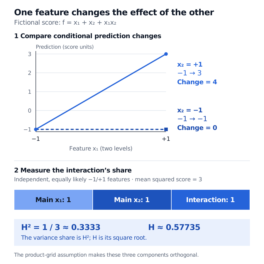
Fictional model f equals x1 plus x2 plus x1 times x2. Changing x1 from minus one to plus one changes the prediction by zero when x2 is minus one and by four when x2 is plus one. Independent equally likely feature levels give mean squared prediction three and mean squared interaction residual one, so H squared is one third and H is about 0.57735.
Original four-point model. Conditional prediction changes reveal the interaction; orthogonal components on the independent product grid give its one-third variance share.
The interaction is visible before calculating the ratio: moving x1 from −1 to +1 changes the prediction by zero when x2=−1, but by four when x2=+1. A single main-effect curve cannot describe both changes.
On this complete independent grid, the two main effects and the product term are orthogonal, each with variance 1. The interaction therefore accounts for one third of the score variance. The variance share is H2, not H: reporting “57.7% of variance” would confuse the two conventions. Removing the product gives H=0; keeping only the product gives H=1 under these same weights.
Read the denominator as carefully as the numerator
With exact marginal averaging and evaluation under the same independent product distribution, orthogonality gives the familiar 0≤H≤1 interpretation. An empirical residual ratio is not automatically a bounded variance decomposition.
Weak joint variation: if the denominator is zero, the normalised score is undefined. Near zero, small approximation errors can dominate. A large pairwise ratio can describe an interaction with little absolute influence on the complete model.
Dependent features: background substitution can create implausible combinations, such as accounting ratios inconsistent with one another. The score may then reflect extrapolated model behaviour. Values above one can occur; clipping them hides the problem. These limitations are documented in the official hstats guidance.
Finite evaluation: a zero residual on the evaluated points establishes additivity there, not everywhere. Subsampling adds variability, and pairwise averaging can conceal higher-order interactions. Inspect the joint surface as well as its summary.
Keep the prediction scale explicit: an additive log-odds model need not be additive after conversion to probability. Comparisons also need a common reference population and weighting scheme. A constant output shift or nonzero linear rescaling leaves this centred ratio unchanged; a nonlinear transformation need not.
A nonzero H is neither a p-value nor evidence of causal interaction. Model fitting can create interactions absent from the underlying relationship; the original paper's §§8.2–8.3 distinguish these and develop a separate null-reference procedure. For financial applications, compare results across appropriate evaluation periods and examine where the observations support the joint surface.
Friedman, J. H. and Popescu, B. E. (2008), Predictive learning via rule ensembles, §§8.1–8.4: centred partial dependence, pairwise and overall normalisations, spurious interactions and null-reference construction.
hstats authors, Interaction Statistics, “Background”, especially “Partial dependence”, “Overall interaction strength” and “Pairwise interaction strength”, plus “Limitations”. Official documentation checked 1 November 2026.