A fiscal multiplier measures the change in real GDP caused by a specified fiscal policy change, per unit of that change. It turns a new spending or tax measure into an estimate of output relative to the path GDP would have followed without it. For a macro forecast, the inputs are the fiscal policy measure, its timing and the response of real GDP over the same horizon. IMF technical note, Box 1 and Section IV.
The first quarter and the full response
Suppose a fictional government unexpectedly raises its purchases for reasons unrelated to the state of the economy. In the quarter of the shock, purchases are 100 currency units above the path without the measure, and GDP is 80 units above its own no-measure path. Both are real flows for the same quarter, measured at the same fixed prices. Write and for these differences from baseline, with the quarter of the shock. The impact multiplier is
Each additional unit of purchases raises real GDP by 0.8 units that quarter in this scenario. Government purchases enter the expenditure measure of GDP. In the example, the other GDP components together are 20 units below baseline, leaving a net gain of 80. IMF technical note, Box 2.
The cumulative multiplier through quarter divides the total output response by the total purchase response, both measured from the shock through the same endpoint. Here we use undiscounted flows. Ramey and Zubairy, Section 3.2.2.
Extend the example by two quarters. Purchases are 50 above baseline in the next quarter and back at baseline the quarter after. The corresponding GDP gains are 55 and 15. Through quarter 2, the cumulative multiplier is . The last quarter still contributes to the numerator even though its purchase response is zero.
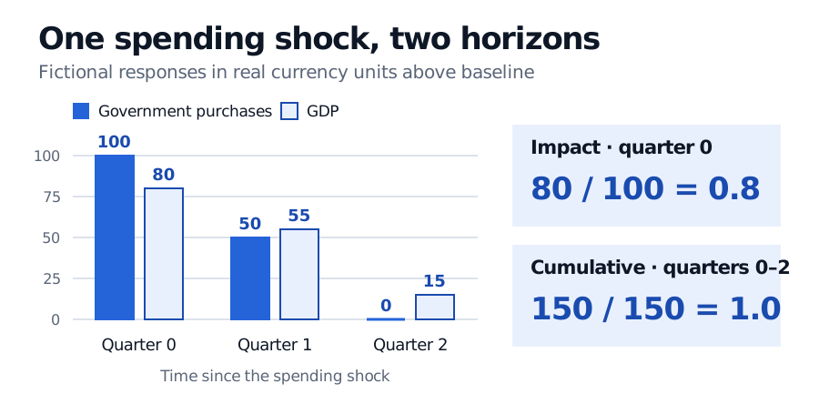
Fictional quarterly responses to one purchase shock, in real currency units above the no-measure baseline. Both cumulative totals include quarters 0 through 2.
Identify the measure before dividing
Use a denominator that matches the intervention. For a cash transfer, use the change in transfer payments. A transfer changes recipients' income, and any spending it induces can affect GDP through consumption. For a tax measure, state the sign convention. Dividing by the positive size of a tax cut gives output gained per unit of tax relief. Dividing by the signed change in taxes reverses that sign. US Bureau of Economic Analysis, government spending measures. IMF technical note, Box 1 and Section II.
In the data, GDP also moves fiscal flows. A downturn can trigger automatic stabilizers, lowering tax receipts and raising some benefits under existing rules. A government may also pass a new package in response to the downturn. Dividing observed changes in GDP and the budget would mix those responses with the effect of policy on output. IMF technical note, Introduction.
One approach is to date the surprise using information available at the time. Valerie Ramey used contemporary reporting on military events to reconstruct revisions to expected US defence spending. Her study found that some conventional estimates dated shocks after the spending news had already arrived. Households and firms can respond when a credible plan becomes known, before purchases begin. If purchases have yet to change in the news quarter, the impact spending ratio has a zero denominator. Ramey, Sections III–V.
Which estimate fits the forecast?
The output response depends on the economy's ability to supply more goods and services, how much new demand goes to imports, and how monetary policy responds. If a central bank raises rates in response to stimulus, weaker interest-sensitive spending can offset some of the GDP gain. Cloyne, Jordà and Taylor document the related mechanism for fiscal tightening. In their sample, the estimated output loss was larger when monetary policy provided less offset. For a forecast revision, use a baseline consistent with what was already expected, then match the estimate to the new measure, the horizon and the assumed monetary response. IMF technical note, Sections II.B and IV. Cloyne, Jordà and Taylor, Section 4.
Sources
- Batini, Eyraud, Forni and Weber (2014), Fiscal Multipliers: Size, Determinants, and Use in Macroeconomic Projections
- Ramey (2011), Identifying Government Spending Shocks: It's All in the Timing
- Ramey and Zubairy, Government Spending Multipliers in Good Times and in Bad
- Cloyne, Jordà and Taylor (2020), Decomposing the Fiscal Multiplier
- US Bureau of Economic Analysis, measures of government spending