Feature hashing: Definition & Examples

Feature hashing maps named input features into a fixed number of numerical columns using a hash function, adding together values that land in the same column. It lets a quant researcher encode an expanding vocabulary of filing terms or categorical identifiers without maintaining a growing feature-to-column dictionary. The price is collisions: unrelated inputs can share a model coefficient.

A fixed address for every feature

Choose an output width $m$ . A bucket function $h(j)$ assigns feature $j$ to one of those columns. Signed hashing also assigns a sign $s(j)\in\{-1,+1\}$ . For input vector $x$ , the value in bucket $b$ is

\phi(x)_b=\sum_{j:h(j)=b}s(j)x_j.

Only nonzero input features need processing, and the output can remain a sparse matrix. New names receive addresses without fitting a vocabulary. Keep the same mapping during training and prediction: changing its hash, seed where configurable, output width or feature naming changes what the model's columns mean. The scikit-learn user guide explains the dictionary-free representation and its loss of inspectability.

A conventional hash table retains keys so it can distinguish them after a collision. Feature hashing deliberately merges their numerical contributions. It is a lossy representation, rather than a way to retrieve the original records.

Follow one collision

Consider three fictional features with counts

x=(2,3,4)

. The following bucket and sign assignments are given for illustration; they are not outputs from MurmurHash3, Python or any library.

Feature	Count	Bucket	Sign	Contribution
A	2	0	$+1$	$+2$
B	3	0	$-1$	$-3$
C	4	1	$+1$	$+4$

The result is $\phi(x)=(-1,4)$ . Its squared length is $(-1)^2+4^2=17$ , whereas the original squared length is $2^2+3^2+4^2=29$ .

Illustrative counts A equals 2, B equals 3 and C equals 4. A maps to bucket 0 with sign plus 1, B to bucket 0 with sign minus 1 and C to bucket 1 with sign plus 1. The encoded vector is minus 1, 4; squared norm falls from 29 to 17.

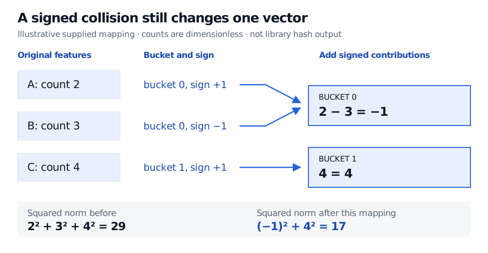
Figure: A supplied mapping, not real library hash output. A and B share a coordinate and partially cancel; their original counts cannot be recovered from the two bucket values.

B has a positive original count. Its negative contribution comes from the encoding convention, not from a negative financial observation. Nor does partial cancellation restore the two original axes.

What the signs preserve

For fixed vectors $x$ and $y$ , independent unbiased random signs, independent of the bucket assignments, are sufficient to give

\mathbb{E}_{h,s}\!\left[\phi(x)^\top\phi(y)\right]=x^\top y.

The expectation is over the random mapping, not over market observations. In the expanded dot product, each feature's own contribution survives because

s(j)^2=1

; cross-feature collision terms average to zero. Weinberger et al. develop this unbiasedness result and stronger concentration results with additional conditions.

The toy makes the distinction concrete. Hold its buckets fixed and draw independent fair signs. A and B have the same sign half the time, giving squared length

5^2+4^2=41

. They have opposite signs half the time, giving

1^2+4^2=17

. The mean is

(41+17)/2=29

. Neither possible squared length equals 29. Randomness balances the collision error across mappings; it does not remove the loss in one deployed mapping. Larger bucket counts trade a larger coefficient vector for fewer collisions; they do not guarantee collision-free data.

Using it with financial text

Hashing chooses coordinates; it does not learn that “impairment” and “write-down” have related meanings. A shared bucket is accidental similarity. It also does not decide how to tokenize a filing, which n-grams to include or whether to scale counts. Use explicit names such as issuer=ABC and venue=ABC when identical strings represent different variables.

The current FeatureHasher API documents signed 32-bit MurmurHash3, a stateless transformation and alternate_sign=True by default. Signed outputs can be negative, so check compatibility with downstream methods requiring nonnegative inputs. The hasher itself does not tokenize text; the user guide distinguishes it from the combined text-processing vectorizer.

Dictionary-free encoding also leaves the research cutoff intact: a filing must have been available when its features were used. Choosing the bucket count or preprocessing after examining future evaluation outcomes can still contaminate the comparison. For the next step, the Text Classification lesson connects representations to labelled financial documents and held-out evaluation. Its public page is a preview; the full lesson requires membership.

Sources

Weinberger, Dasgupta, Attenberg, Langford and Smola, Feature Hashing for Large Scale Multitask Learning, sections 2–3. Original 2009 paper; revised version dated 27 February 2010.
scikit-learn, Feature hashing user guide, including implementation details.
scikit-learn, FeatureHasher API reference, parameters and notes. Official software documentation checked 1 November 2026.

A fixed address for every feature

Follow one collision

What the signs preserve

Using it with financial text

Sources

Related terms

Dot product

Hash table