Exponential smoothing is a family of forecasting methods that recursively updates estimates of a time series’ level, trend or seasonal pattern as observations arrive. Its simplest form gives a quant a transparent baseline: forecast the next observation from the current level, then adjust that level by a fraction of the forecast error.
Two numbers with different information dates
In simple exponential smoothing (SES), let be the observation and the level after observing it. With smoothing weight ,
The first number is available before ; the second incorporates it. SES has no trend or seasonal component. From a fixed origin , every future point forecast is for . Flat point forecasts do not imply certain future outcomes. These mechanics are set out in Hyndman and Athanasopoulos, §8.1.
Take the fictional observations 10, 14, 12, 20 index points, set , and initialise . Begin updating at period 2:
The forecast for period 4 was 11.25. Its error is points; only then does the level rise by points. 13.4375 is the forecast for period 5. Scoring it against period 4 would give the forecasting procedure information from its own target.
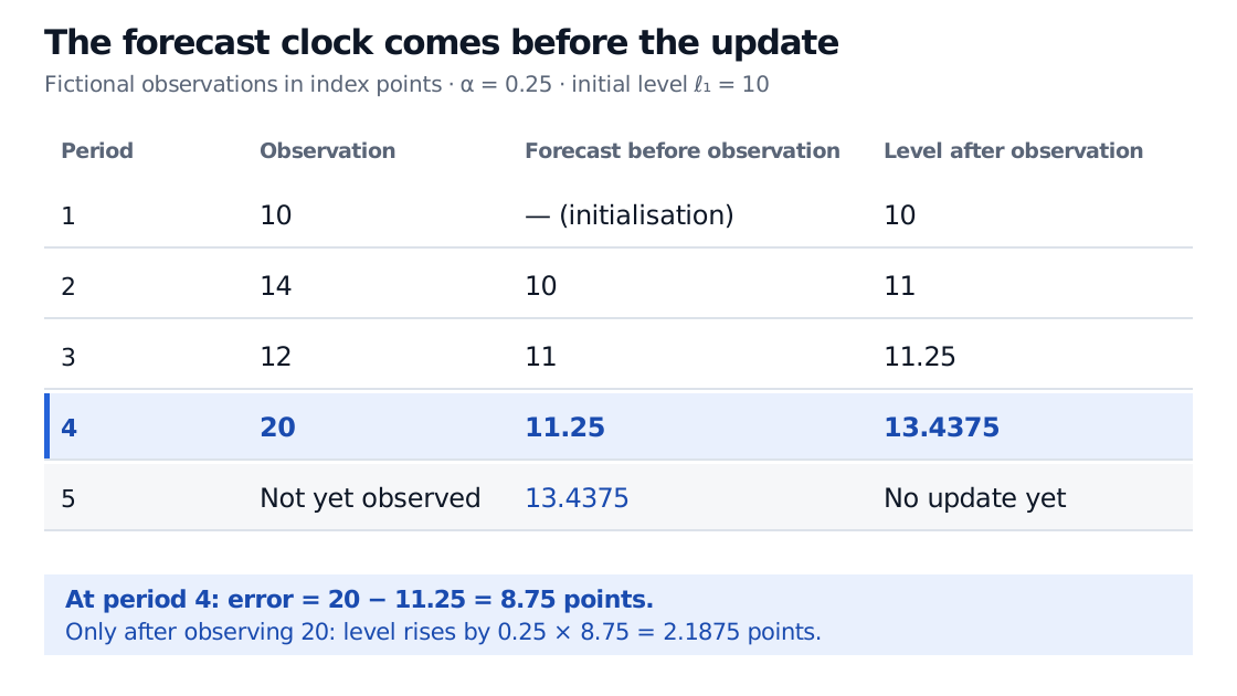
The forecast uses the previous level. The updated level becomes available only after the target observation arrives.
Initialising at the first observation is a stated convention for this example, not a forecast made before period 1. If parameters or initial states are fitted using a training sample, its one-step fitted values also depend on that estimation sample. An honest later test must respect both the state-update clock and the parameter-selection clock. The Forecast Evaluation lesson develops chronological testing and loss comparisons; its preview is public and the full lesson requires membership.
“Exponential” includes an initialisation remainder
Unroll our particular recursion:
These weights add to one. Because , the last term contributes 4.21875 points, almost a third of the final level. It would be a material error to drop it after only three updates.
More generally, with this initialisation at period 1,
The geometrically declining observation weights connect SES to time-decay weighting. The finite recursion retains the initial state’s remaining weight; an infinite-history expression suppresses that boundary. FPP, second edition, §7.1 presents the corresponding finite expansion using an initial state at time 0.
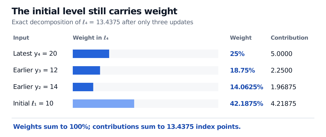
The initial state carries the history before the recursive updates begin; it is not assigned the same coefficient as an ordinary later observation.
Larger makes the level react more strongly to new information; smaller retains more of the previous state. At , the next forecast is the latest observation; at , the level never updates. No coefficient is universally best: evaluate the chosen horizon and loss on later data.
Choose the component and the target
SES smooths a level. Holt’s linear method adds a trend state , giving forecasts ; a damped trend attenuates its extrapolation. Holt–Winters adds seasonal states. Additive seasonality describes roughly constant-sized seasonal movements, whereas multiplicative seasonality describes movements proportional to the level. Changing alone cannot add these missing components. See FPP, second edition, §§7.2–7.3.
An EWMA volatility forecast instead updates a variance using squared return shocks. Its decay parameter often weights the old state, so can play the role of . Similar recursion does not make a smoothed price level a volatility estimate—or establish profitable price predictability.
Practice: freeze the forecast
A fictional series has current level 8 points and . Before the next observation arrives, you issue its one-step forecast. The observation is then 13 points. What was the issued forecast, and what forecast can you issue for the following period?
Answer. The issued forecast was 8. The error is , so the new level is points. The following period’s forecast is 10. Reporting 10 as the earlier forecast would use the later observation.
Sources
- Hyndman, R. J., and Athanasopoulos, G., Forecasting: Principles and Practice, third edition, Chapter 8, especially §8.1 on SES, flat forecasts and initialisation, and §8.5 on the distinction between point-forecast methods and stochastic models.
- Hyndman, R. J., and Athanasopoulos, G., Forecasting: Principles and Practice, second edition, Chapter 7, §§7.1–7.3 on finite weights, trend and seasonal extensions. Examples, calculations and figures above are original.