Evidential deep learning: Definition & Examples

Evidential deep learning (EDL) trains a neural network to output the parameters of a distribution over possible predictive distributions. In classification, this adds a distribution over class probabilities to the class prediction itself. For a quant classifying default events or market states, the appeal is an uncertainty score available from one network evaluation. Whether that score identifies unreliable forecasts must still be tested.

What the classifier outputs

In the classification construction of Sensoy, Kaplan and Kandemir (2018), Sections 3–4, the network produces non-negative evidence values

e_k(x)

for

K

mutually exclusive classes. These determine a Dirichlet distribution:

\alpha_k=e_k+1,\qquad S=\sum_{k=1}^{K}\alpha_k,\qquad p\mid x\sim\operatorname{Dirichlet}(\alpha_1,\ldots,\alpha_K).

The vector $p$ contains class probabilities that sum to one. Conditional on $p$ , the next label follows a categorical distribution. Averaging over $p$ gives predictive class probabilities

\hat p_k=\mathbb E[p_k\mid x]=\frac{\alpha_k}{S}.

Under the paper's subjective-logic convention, singleton belief masses and the remaining uncertainty mass are

b_k=\frac{e_k}{S},\qquad u=\frac{K}{S},\qquad \sum_{k=1}^{K}b_k+u=1.

Thus $\hat p_k=b_k+u/K$ . Belief mass $b_k$ alone is not the predictive class probability. Here, “evidence” is learned support output by the network; it is not automatically a count of independent observed events, nor the marginal likelihood also called evidence in Bayesian inference.

A 60% prediction has more than one possible concentration

Consider a stipulated binary classifier output, not a trained financial model. Class one could denote a default within a specified horizon; class two denotes no default. Let the evidence be

e=(2,1)

. Then

\alpha=(3,2),\qquad S=5,\qquad \hat p=(0.6,0.4).

The belief masses are $b=(0.4,0.2)$ and $u=2/5=0.4$ . Each class receives $u/2=0.2$ in the predictive mean. The result is internally consistent, but it supplies no empirical default-frequency evidence.

The variance of the probability $p_1$ under this Dirichlet output is

\text{Var}(p_1\mid x) =\frac{\alpha_1(S-\alpha_1)}{S^2(S+1)} =\frac{3\times2}{25\times6}=0.04.

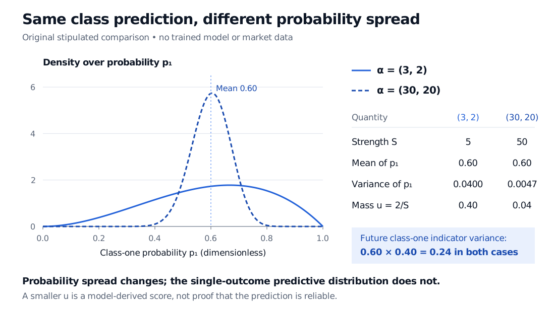
Now stipulate a second output $\alpha=(30,20)$ , corresponding to evidence $(29,19)$ . It has the same predictive mean, but $S=50$ , $u=0.04$ , and probability variance $0.24/51\approx0.004706$ . The network has expressed a much more concentrated opinion without changing its 60% class-one prediction.

Two stipulated binary evidential outputs have the same mean class-one probability 0.60. Parameters 3 and 2 give strength 5, probability variance 0.0400 and uncertainty mass 0.40. Parameters 30 and 20 give strength 50, probability variance about 0.0047 and mass 0.04. Both imply future class-one indicator variance 0.24.

Original stipulated distributions, not fitted financial forecasts. For two classes the Dirichlet reduces to a Beta density for p₁. Concentration changes without changing the single-outcome class probabilities.

The variance of the probability is not the variance of the next outcome. Define

Y=1

when class one occurs and

Y=0

otherwise. After integrating out

p_1

, both examples give

Y\sim\operatorname{Bernoulli}(0.6)

, so

\text{Var}(Y\mid x)=0.6(1-0.6)=0.24.

For the first output, the law of total variance makes the distinction explicit:

\begin{aligned} \text{Var}(Y\mid x) &=\mathbb E[p_1(1-p_1)\mid x]+\text{Var}(p_1\mid x)\\ &=0.20+0.04=0.24. \end{aligned}

This decomposition follows from the specified hierarchy. Calling its second term epistemic uncertainty does not establish that it faithfully measures the learner's actual lack of knowledge.

The learning objective matters

Predicting Dirichlet parameters does not specify how to learn them. The original classification paper considers several losses and selects expected squared error under the Dirichlet, adding an annealed KL penalty intended to discourage misleading evidence. The concentration therefore depends on training choices as well as labels. This is a different construction from a Bayesian neural network, which models uncertainty over network parameters.

Jürgens and coauthors (2024), Sections 3–5, analyze several second-order loss constructions. They identify non-identifiability for unregularized inner loss minimization: different Dirichlet concentrations can produce the same categorical predictive distribution. For unregularized outer losses they establish collapse results under stated assumptions; regularization changes the behavior but does not generally recover their reference uncertainty distribution. Their reference is based on refitting first-order learners across resampled datasets, and depends on the learner and fitting procedure.

These findings do not say that every EDL score is useless. They distinguish useful relative ranking of unfamiliar inputs from faithful quantitative uncertainty. In particular,

u=0.4

does not mean a calibrated 40% probability that the model is wrong, nor does a small

u

guarantee that an input belongs to the training distribution.

For a financial application, evaluate the mean probabilities on later eligible observations and examine whether high- $u$ cases actually have worse errors or useful rejection behavior. Compare retained-sample error together with the fraction of predictions retained; rejecting almost everything can make accuracy look good. Keep overlapping label horizons and information available at the decision time in the validation design. Test changed market conditions explicitly rather than assuming that unfamiliar conditions must raise $u$ .

The Probability calibration lesson develops the distinction between ranking and probability reliability before scores enter position sizing. Its preview is public; the full lesson requires membership. Calibration of

\hat p

does not, by itself, validate the separate concentration score.

Regression uses a different hierarchy

Amini and coauthors' Deep Evidential Regression, Section 3, instead predicts normal–inverse-gamma parameters over the mean and variance of a Gaussian observation model. Integrating those parameters produces a Student's

t

predictive distribution. Its parameters, moment conditions and uncertainty formulas differ from the classification construction:

K/S

is not a general evidential-regression formula. A return forecast using that model also inherits the Gaussian conditional-observation assumption; the method's name alone does not justify it for a chosen financial target.

Sources

Sensoy, Kaplan and Kandemir (2018), Evidential Deep Learning to Quantify Classification Uncertainty, Sections 3–4: classification evidence, Dirichlet opinions and training objectives.
Jürgens, Meinert, Bengs, Hüllermeier and Waegeman (2024), Is Epistemic Uncertainty Faithfully Represented by Evidential Deep Learning Methods?, Sections 3–5: reference distributions, identifiability, optimization and limits of quantitative uncertainty interpretations.
Amini, Schwarting, Soleimany and Rus (2020), Deep Evidential Regression, Sections 3.1–3.3: the normal–inverse-gamma hierarchy and predictive distribution.

What the classifier outputs

A 60% prediction has more than one possible concentration

The learning objective matters

Regression uses a different hierarchy

Sources

Related terms

Bayesian neural network

Neural network