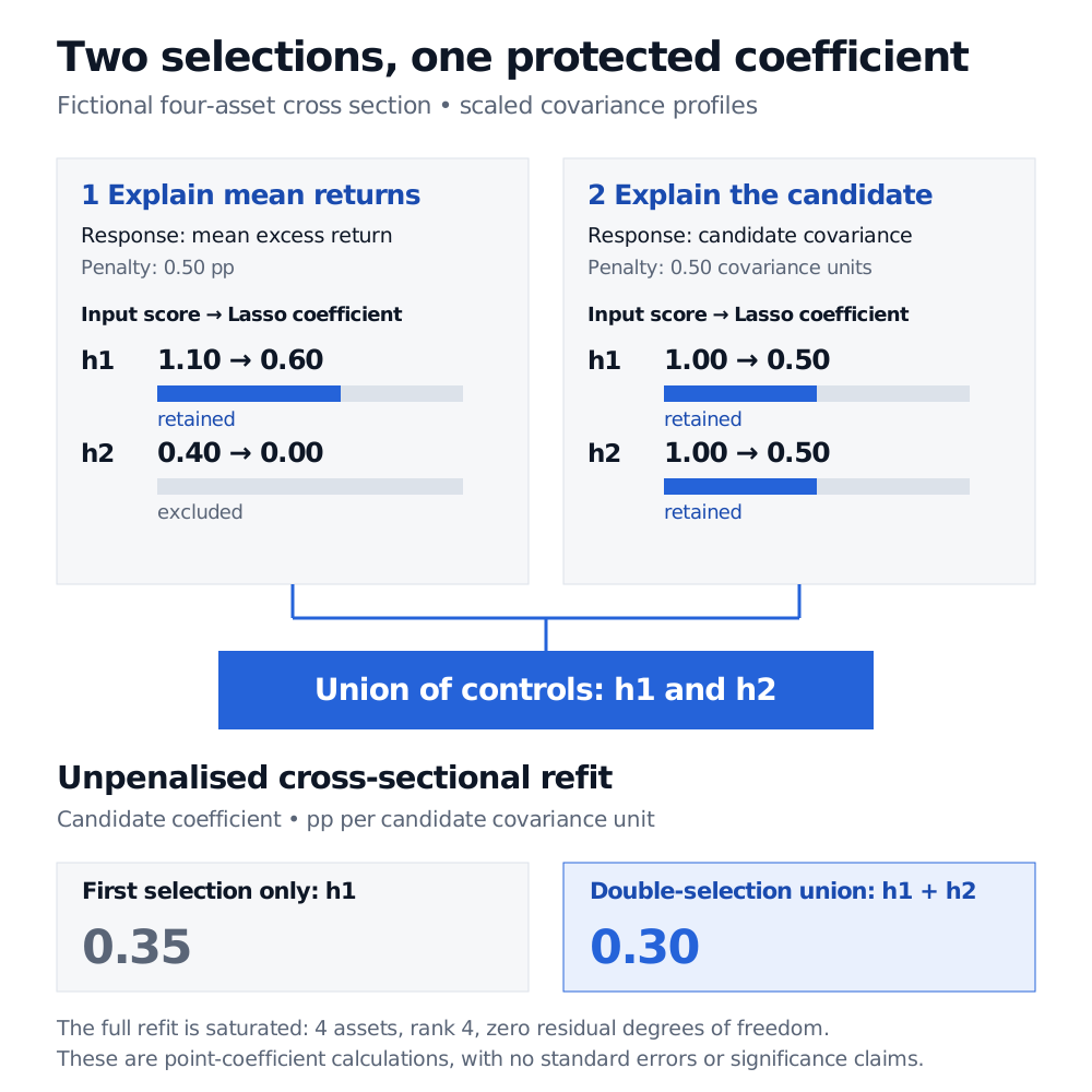
Double-selection LASSO tests a new factor against many controls by selecting for both mean returns and candidate covariances before an unpenalised refit.
Double-selection LASSO
Double-selection LASSO is a control-selection procedure that screens a large factor set twice before estimating the incremental pricing contribution of a candidate factor. In the Feng–Giglio–Xiu asset-pricing application, the two screens protect against a specific mistake: discarding a control that contributes modestly to explaining average returns but materially changes the candidate factor’s coefficient when omitted.
A factor surviving ordinary Lasso regression is not, by that fact alone, an independently priced source of risk.
Two questions for the same control set
Let rt contain returns on n test assets, gt be one candidate factor and ht the existing factor set. Write Cg=Cov(rt,gt) and Ch=Cov(rt,ht). In the covariance representation,
E[rt]=1γ0+Cgλg+Chλh.
The target λg is the candidate’s stochastic discount factor loading, rather than its mean return or its multivariate-beta risk premium. Those parameters can differ when factors are correlated.
Using sample means and covariances, the procedure is:
Select for pricing: regress average asset returns on existing-factor covariance columns using Lasso. Keep the selected set Sy.
Select for overlap: regress the candidate’s covariance column on the same controls using a second Lasso. Keep Sg.
Refit: regress average returns on the candidate covariance column and the controls in Sy∪Sg, with an intercept and without a penalty.
These are cross-sectional regressions across test assets. The second screen compares covariance profiles; it is not a regression of factor returns through time. Feng, Giglio and Xiu, §I.E, equations (7)–(9).
A control that the first screen misses
Consider four fictional assets. The inputs below are stipulated, scaled covariance profiles and average excess returns over a common, unspecified horizon. They are not four dates of factor returns or sample estimates from a simulated return panel.
Asset
Control profile h1
Control profile h2
Candidate profile cg
Mean excess return y (pp)
A
−1
−1
−3
−1.8
B
−1
1
1
−0.4
C
1
−1
1
1.0
D
1
1
1
1.2
Here h1,h2 name the columns of the scaled control covariance matrix, rather than the underlying factor time series. Construct a third orthogonal column u=(−1,1,1,−1)⊤ and set
cg=h1+h2+u,y=0.8h1+0.1h2+0.3cg.
All columns are centred. For C=(h1h2), C⊤C/4=I, and C⊤u=0. Use the explicit Lasso convention
a,bmin2n∥q−a1−Cb∥22+ℓ∥b∥1,n=4,
where the intercept a is unpenalised. The symbol ℓ denotes the tuning penalty, keeping it distinct from the pricing loading λg.
For these orthonormal controls, let z=C⊤q/n. Each coefficient is soft-thresholded:
bj=sign(zj)max(∣zj∣−ℓ,0).
For the first response, q=y, the scores are (1.1,0.4). A penalty ℓy=0.5 pp gives coefficients (0.6,0): only h1 survives. The scores follow from y=1.1h1+0.4h2+0.3u, not from reading off the structural control coefficients 0.8 and 0.1.
For the second response, q=cg, the scores are (1,1). A separately specified penalty ℓg=0.5 in candidate covariance units gives (0.5,0.5): both controls survive. The two numerical penalties happen to match; their response units differ. They are illustrative tuning choices, not a prescription for empirical work.
Fictional four-asset covariance example: mean-return Lasso coefficients are 0.60 and 0 for h1 and h2; candidate-covariance Lasso coefficients are 0.50 and 0.50. The union retains both controls, giving a candidate coefficient of 0.30 versus 0.35 with h1 alone. The saturated full refit supplies no statistical inference.
Original synthetic selection geometry. The two Lasso responses have different units and separately specified penalties; the final coefficient is in percentage points per candidate covariance unit. No estimated time series or significance test is represented.
The union therefore includes h2. The unpenalised ordinary least-squares refit recovers the stipulated candidate coefficient 0.30, in pp per candidate covariance unit.
Keeping only the first selection produces 0.35. To see exactly why, remove the component along h1 from the candidate and response. The remaining vectors are h2+u and 0.4h2+0.3u, giving
After also controlling for h2, the remaining vectors are u and 0.3u, giving 0.30. The omitted h2 raises the first coefficient by 0.05: a concrete omitted-variable bias mechanism, even though the first screen excluded it.
The full design has four assets and four linearly independent columns, counting the intercept. It is saturated, with zero residual degrees of freedom. This calculation demonstrates selection geometry and point estimates; it provides no standard error, confidence interval or p-value.
What turns selection into inference?
The final paper’s §I.F uses jointly large asset and time dimensions, sparsity and further regularity conditions. Its asymptotic distribution is scaled by T, and its variance estimator is Newey–West-type. Computing that variance also involves a separate time-series Lasso/post-OLS projection of gt on ht; that is not the second cross-sectional selection above. Merely attaching ordinary regression standard errors to the union refit does not implement this framework. Feng, Giglio and Xiu, Theorems 1–2 and equation (10).
The original Belloni–Chernozhukov–Hansen post-double-selection framework concerns treatment effects in approximately sparse models. Its causal interpretation requires its own identifying assumptions. Selecting controls twice does not make an asset-pricing coefficient a causal effect.
Double/debiased machine learning is a broader framework using orthogonal scores and cross-fitting; it is not simply another name for two Lasso fits. Chernozhukov and coauthors. Likewise, searching many candidate factors and reporting the best result introduces a separate multiple-testing problem. Double selection targets the choice of controls for a factor under evaluation.