DeepLIFT attributes a change from a reference; LRP redistributes a selected model score. Compare finite differences, signed relevance and conservation with two separate worked examples.
DeepLIFT and layer-wise relevance propagation
DeepLIFT and layer-wise relevance propagation (LRP) are methods for assigning a fitted model's prediction to its inputs by sending attribution signals backward through its computation. For a quant analysing a neural network, they can reveal which features support or offset a particular forecast. Their answers depend on the output being explained and the attribution rules.
DeepLIFT means Deep Learning Important FeaTures. It explains a change from a chosen reference input. LRP redistributes a chosen output score through successive layers. A sum of attributions is an accounting identity under specified rules; it does not establish causal effects.
DeepLIFT: explain the move from a reference
For a scalar target f, input x and reference x0, DeepLIFT seeks contributions satisfying
i∑Ci=f(x)−f(x0).
Reference activations are obtained by passing the reference input through the same network. Multipliers propagate contributions using a chain rule. Different nonlinear rules, including Rescale and RevealCancel, need not give the same attribution. Shrikumar, Greenside and Kundaje define these rules and the summation-to-delta property in §§3.1–3.5.
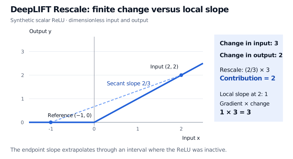
Consider the synthetic, dimensionless scalar model y=max(0,x), a ReLU. Use the Rescale rule, reference x0=−1 and input x=2. The reference output is zero and the target output is two:
Δx=2−(−1)=3,Δy=2−0=2.
The Rescale multiplier is the secant slope across this interval:
m=ΔxΔy=32,C=mΔx=2.
At the target, the ordinary derivative is f′(2)=1. Multiplying this local slope by the same input change gives 1×3=3, which overstates the actual output change. One unit of the input interval lies below zero, where the ReLU is inactive. The endpoint derivative does not capture that part of the journey.
A synthetic ReLU has reference input minus 1 with output 0 and target input 2 with output 2. The input change is 3, the secant multiplier is two thirds, and the DeepLIFT contribution is 2. The local gradient times the input change is 3.
Original synthetic DeepLIFT Rescale example. The dashed secant spans the reference and input; the solid curve is the ReLU. All quantities are dimensionless.
Changing the reference changes the question: with reference x0=1, the same model at the same input has output change 2−1=1. Neither reference is universally neutral. In a financial feature vector, zero might mean the training mean after standardisation, while a zero raw spread or zero price means something very different.
LRP: distribute a score through the layers
LRP starts with relevance assigned to a selected output. For a bias-free layer, the basic z-rule redistributes relevance Rj using forward contributions zij=aiwij:
Ri=j∑∑kzkjzijRj.
Here ai is an input activation and wij its connection weight; the denominators must be nonzero. The fractions sum to one for each receiving unit, conserving its relevance. Bach et al. describe the conservation principle and propagation variants, including bias and stabilisation handling.
Use a separate synthetic linear model,
f(x1,x2)=2x1−x2,(x1,x2)=(3,1).
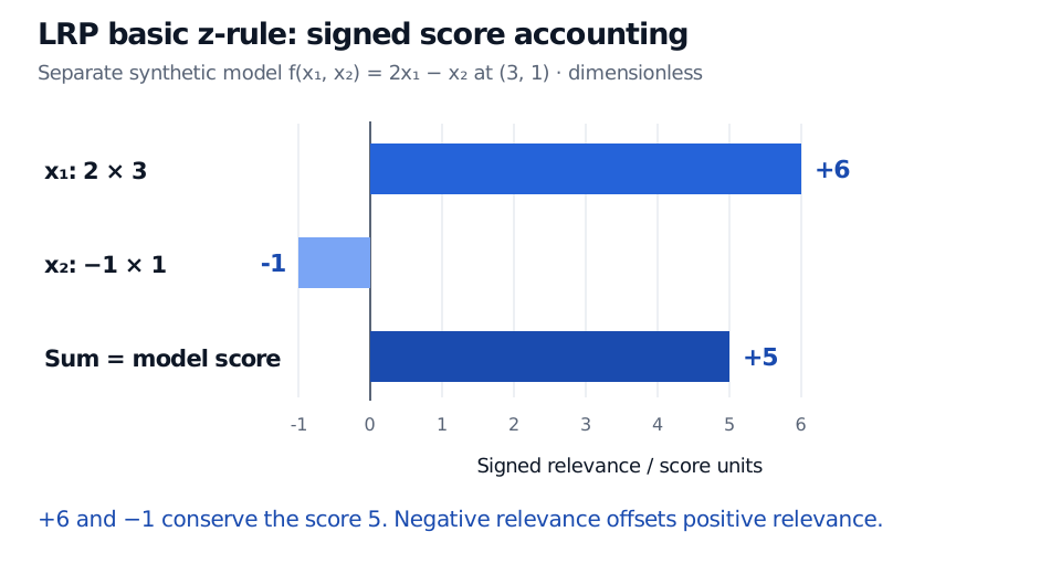
There is no bias. Initialise output relevance to the dimensionless score Rout=f(3,1)=5. With forward contributions six and minus one, the basic z-rule gives
R1=56×5=6,R2=5−1×5=−1.
The signed sum is five. A feature can receive relevance larger than the total because another offsets it. Taking absolute values would give seven and destroy this accounting. These are score units, not percentages or probabilities.
A separate linear LRP example has first-feature relevance plus 6, second-feature relevance minus 1, and total relevance 5, equal to the model score.
Original synthetic LRP basic z-rule example with no bias and a nonzero denominator. Signed contributions conserve the dimensionless score; their absolute magnitudes do not.
Near cancellation, the basic denominator can be tiny and individual relevances can become large. Epsilon-LRP adds a stabiliser to the denominator. It can absorb relevance, so exact conservation requires explicit residual accounting or redistribution. Bias terms also require a declared convention. Positive-only and other propagation rules change what is allocated; “LRP” alone does not fully specify an explanation.
Read a financial attribution as a model diagnostic
Record the target first: a return forecast, a class logit and a class probability have different scales. A logit attribution cannot be relabelled as a probability-point contribution. For DeepLIFT, also record the reference, preprocessing and nonlinear rule. For LRP, record the layer rules, bias treatment, stabiliser and any unallocated residual.
Correlated financial features can share information. A large attribution to a volatility feature may describe a shortcut learned from a particular training period; it does not show that intervening on volatility would produce the attributed return. Compare explanations across sensible reference scenarios and time periods before treating a feature ranking as stable.
Gradient saliency instead measures local sensitivity. Integrated gradients integrates gradients along a reference-to-input path, whereas DeepLIFT uses layer-specific contribution rules. Captum's algorithm descriptions distinguish these constructions. Agreement in a simple model does not make the methods interchangeable in an arbitrary network.
For the derivative machinery behind these comparisons, see Backpropagation as the Chain Rule (public preview; full lesson requires membership).