Deep Sets pool shared element representations to make a prediction invariant to row order. Trace sum pooling, multiplicity and the limits of universality.
Deep Sets and permutation-invariant networks
Deep Sets is a neural-network architecture for collections whose output should remain unchanged when their input rows are reordered. It applies a shared transformation to every element, pools the resulting representations, then maps the pooled representation to an output. In quant work, this can stop an arbitrary database row order from changing a prediction about a holdings snapshot. It does not establish that the chosen financial data should be treated as unordered.
A shared map, a sum, a readout
The basic sum-pooling form is
f(x1,…,xn)=ρ(i=1∑nϕ(xi)).
Here xi can be a vector of features. The same map ϕ transforms each element into a latent feature vector, and ρ produces the final output. In a learned model, these maps are typically neural networks. Their parameters are shared across the elements, rather than assigned according to row position. Wagstaff and colleagues, Figure 1, illustrate this sum-decomposition structure.
Addition preserves the total when its terms are reordered, so the readout receives the same vector. Permutation invariance concerns one output for the whole collection. Permutation equivariance concerns outputs attached to individual elements: reorder the inputs, and those outputs reorder correspondingly. A portfolio-level score and one score per holding therefore require different output structures. The distinction is formalised in the original paper, §2.1.
What survives the shuffle
Use fixed, hand-chosen maps to isolate the mechanism:
ϕ(x)=(x,x2),ρ(a,b)=a+0.1b.
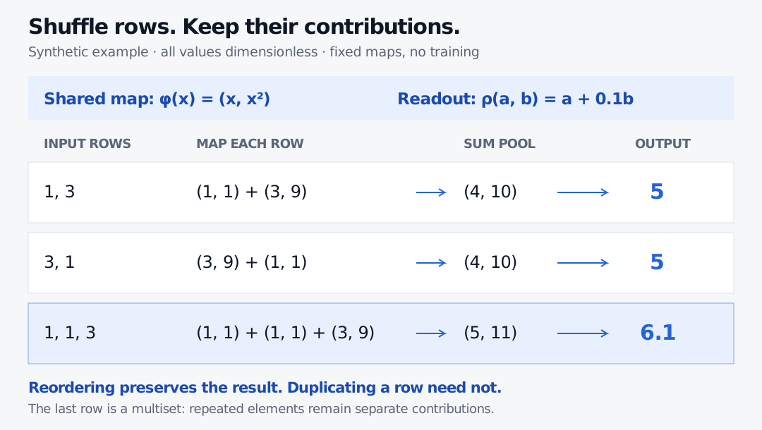
All values are dimensionless. For the two input rows 1,3, the shared map produces (1,1) and (3,9). Their sum is (4,10), giving
f(1,3)=4+0.1(10)=5.
Reversing the rows produces exactly the same pooled vector and output. These are stipulated computations, with no training or forecast interpretation.
The input rows 1,3 and 3,1 both map and sum to (4,10), giving output 5. The multiset 1,1,3 instead sums to (5,11), giving 6.1.
Original synthetic calculation with fixed maps and dimensionless values. Reordering leaves the sum unchanged; adding a second copy of 1 changes the pooled vector and output.
Adding another 1 creates the multiset1,1,3: unlike a mathematical set, a multiset retains repeated elements. The pooled vector becomes (5,11) and the output is 5+0.1(11)=6.1. Invariance to order is not indifference to multiplicity or collection size. Sum pooling can preserve count explicitly by including a constant feature ϕ0(x)=1, whose pooled value is n.
Mean pooling changes what is retained. Averaging these mapped vectors gives (2,5) for both 1,3 and 1,1,3,3. Duplicating the whole collection changes its size but leaves its mean representation unchanged. If count matters, mean pooling alone loses that distinction; count must reach the readout through another feature or input. Conversely, sum pooling does not automatically distinguish every different collection: the information retained depends on the chosen map.
Invariance is easier than universality
The sum architecture guarantees order invariance algebraically. Claims about representing every invariant function need stronger assumptions. The original paper's Theorem 2 concerns a countable element universe; it explicitly separates the uncountable case and fixed-size results. These qualifications matter for real-valued features. See Zaheer et al., §2.2.
Wagstaff et al., §§3–4, examine continuous mappings, which are central to practical neural implementations. In their scalar-element setting, representing arbitrary continuous invariant functions on collections of size up to M requires latent dimension at least M. Their variable-size result also specifies a notion of continuity across sizes. This is a universality requirement, not a claim that every useful function needs that width: §4.1 explicitly distinguishes the two. A fixed small latent vector is therefore not a universal guarantee for arbitrarily large collections, and a representation theorem does not guarantee that training will find a useful model.
Which finance inputs are actually unordered?
An illustrative use is a model receiving one row per position at a common valuation time. Reordering those same complete rows should not alter a portfolio-level output. Each row must include the economically relevant position weight or quantity and security features; feeding only security names discards information about the actual exposure. Splitting a position into multiple rows is a change in representation, not a permutation, so its treatment needs a separate design decision.
An event stream is different. Permuting transactions can remove timing and execution dependencies. Pooling counterparties without encoding their relationships can remove graph structure relevant to the task; a graph neural network addresses a different input structure. Adding timestamps or relationship features may retain some information, but invariance alone does not recover omitted structure.
For the temporal alternative, Recurrent Networks for Structured Data derives a state update in which earlier inputs affect later ones. Its preview is public; the full supporting Library lesson requires membership. Choose the symmetry from the economic question before choosing the pooling operation.
Sources
Manzil Zaheer and colleagues, Deep Sets, NeurIPS 2017. §§2.1–2.2 define invariance and equivariance and state the representation result with its domain qualifications; §3.1 introduces the architecture.
Edward Wagstaff and colleagues, On the Limitations of Representing Functions on Sets, ICML 2019. §3 explains why continuity matters; §4, Theorems 4.1, 4.3 and 4.4, and §4.1 establish and interpret latent-dimension conditions. The arithmetic example and finance illustrations above are original.