DeepIV learns a treatment distribution and integrates a nonlinear response over it. See why predicting mean treatment is insufficient and valid instruments remain essential.
Deep instrumental variables
Deep instrumental variables, usually called DeepIV, is a two-stage method that uses neural networks to estimate a nonlinear structural response with valid instrumental variables. Its defining step is to average candidate responses over a conditional treatment distribution, rather than feed a predicted mean treatment into an ordinary outcome model. For a quant studying the cost of an execution decision, this distinction separates a possible intervention response from a pattern generated by traders choosing actions when conditions change.
What the two networks learn
Write Y for the outcome, T for the treatment, X for observed controls and Z for excluded instruments. A simplified additive structural model is
Y=h(T,X)+ε,E[ε∣X,Z]=0.
The treatment can still be endogenous: E[ε∣T,X] need not vanish. Taking conditional expectations gives the identifying equation
E[Y∣X=x,Z=z]=∫h(t,x)dF(t∣x,z).
The first network estimates F(T∣X,Z): probabilities for discrete treatments or a conditional density for continuous ones. The second represents hθ and minimises an integrated squared-error objective such as
n1i=1∑n(Yi−∫hθ(t,Xi)dF(t∣Xi,Zi))2.
The excluded instrument enters the treatment distribution, not the structural response as an additional direct predictor. Hartford et al. (2017), §§2–3, introduce this DeepIV construction. Integration is exact for small discrete supports; continuous-treatment implementations can sample from the fitted distribution.
Why the mean treatment loses information
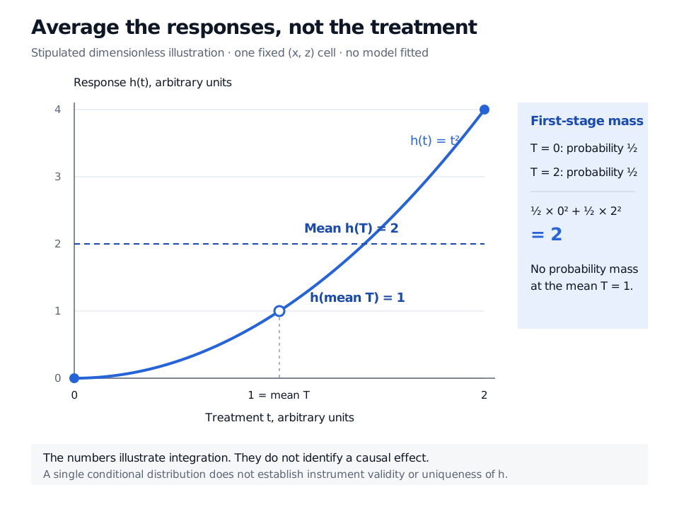
Fix one particular (x,z) cell. Stipulate, without fitting any data, that T=0 or T=2, each with probability 1/2, and that the candidate response is h(t)=t2. Then
E[h(T)∣x,z]=21(02)+21(22)=2,h(E[T∣x,z])=h(1)=1.
The gap is the treatment variance: E[T2]−(E[T])2=1 in this cell. Averaging treatment first discards the dispersion that the nonlinear response reacts to. With a response linear in treatment, the two operations agree; that property does not survive an arbitrary nonlinear second stage.
Stipulated treatment T is 0 or 2 with equal probability. For h(t) = t squared, averaging the responses gives 2, whereas evaluating the response at mean treatment 1 gives 1. This is an integration illustration, not an estimated causal effect.
Original dimensionless illustration: the entire conditional treatment distribution enters the response integral. The midpoint has no treatment probability mass in this example.
These numbers illustrate the integration step only. They are neither fitted DeepIV outputs nor an identified causal effect. The stipulated midpoint response is not observed: this distribution assigns no mass to T=1. Moreover, in this one cell the constant candidate h(t)=2 produces the same integrated response as the quadratic. An average of 2 alone cannot select between them. Identification needs informative variation across instruments and assumptions about the admissible functions.
An execution question needs an instrument argument
Consider a hypothetical broker studying how a trader's chosen participation-rate cap affects implementation shortfall. Traders may choose higher caps when they expect adverse price moves. Hidden urgency then influences both the action and its outcome; accurately predicting shortfall from chosen caps does not remove that selection.
A randomly assigned interface default could be proposed as an encouragement instrument. Before using it, the researcher must defend three separate claims:
Relevance: the default changes the distribution of chosen caps after conditioning on the pre-decision controls.
Exclusion: the default affects shortfall only through that cap. If it also changes routing, fees, trader attention or submission delay, this argument fails.
Exogeneity: conditional on the controls, the assignment is independent of the structural disturbance. Assignment triggered by hidden urgency would violate this condition.
This is a proposed research design, not evidence that interface defaults are valid instruments. The outcome horizon, cap definition and execution mechanism must stay consistent with the intervention being studied. A neural network cannot repair a direct default-to-cost channel or an assignment rule linked to private information. The owned Endogeneity and Instrumental Variables lesson develops the linear foundations; its public page is a preview and the full lesson requires membership.
Flexibility does not guarantee identification
Relevance alone is insufficient for an unrestricted response curve. A standard nonparametric identification condition is completeness: within the chosen function class, if
E[a(T,X)∣X,Z]=0,
then a(T,X)=0 almost surely. Otherwise two distinct responses differing by a can generate identical conditional outcome means. This is an analogue of a full-rank condition, not a synonym for a nonzero first-stage correlation. Newey's author slides, identification slides 6–8, explain this distinction.
Even when a response is uniquely identified, recovering it can be an ill-posed inverse problem: conditional averaging smooths away features, so small estimation errors can imply large response changes. Regularisation controls this instability; it also restricts which shapes the fitted network can recover. Sparse instrument-induced variation makes fine nonlinear features especially difficult to learn. Newey's estimation and instrument-strength slides develop these limitations.
In practice, assess the first-stage distribution, response sensitivity and validation design together. Sampling noise in the first stage feeds into the second; a fitted curve by itself supplies no confidence interval. Held-out fit can reveal overfitting, but cannot establish exclusion, completeness or the credibility of extrapolating an intervention outside the informative treatment range.