Learn policies from logged bandit feedback using propensity-weighted loss and variance control; distinguish IPS, SNIPS and the original CRM learning objective.
Counterfactual risk minimisation
Counterfactual risk minimisation (CRM) is a principle for learning a decision policy from logged action–outcome data by balancing estimated loss against the uncertainty introduced by reweighting that log. In execution research, it provides a way to compare candidate order-selection rules when historical records contain outcomes only for the orders actually chosen.
Here, “risk” means expected loss under a policy. It need not mean portfolio volatility, and the named CRM principle is distinct from a generic claim to minimise causal risk.
What the log can tell you
Imagine a fictional execution experiment with two permitted actions: a passive order or an aggressive order. Each decision records the market context xi, chosen action ai, observed loss ℓi, and logging probability pi=π0(ai∣xi). Let loss be an indicator of failing a predefined execution-cost benchmark: zero for meeting it and one for failing it. This bounded score discards the magnitude of any failure.
For a candidate policy π, the ratio
wi(π)=piπ(ai∣xi)
increases a recorded action's influence when the candidate would choose it more often. This is importance sampling. It changes the weight of an observed loss; it does not reveal the unchosen order's loss on that occasion. The setting is a one-step contextual bandit, rather than a complete sequential execution model.
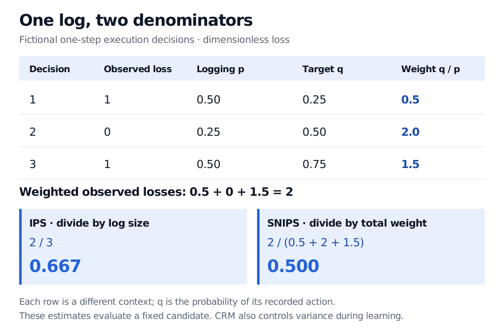
Consider one fixed candidate and three fictional decisions:
Decision
Observed loss
Logging probability of chosen action
Candidate probability of chosen action
Weight
1
1
0.50
0.25
0.5
2
0
0.25
0.50
2.0
3
1
0.50
0.75
1.5
Each row concerns a different context. The candidate probabilities in this column need not sum to one; within each row, probabilities across the two available actions must.
The inverse propensity scoring (IPS) estimate is
RIPS(π)=n1i=1∑nwi(π)ℓi=30.5+0+1.5=32.
The self-normalized IPS (SNIPS) estimate instead divides by the sum of weights:
RSNIPS(π)=∑iwi(π)∑iwi(π)ℓi=42=0.5.
The two denominators answer the same population question through different finite-sample estimators. SNIPS is a weighted average of the observed losses when its denominator is positive; it is generally biased in finite samples. Neither number is the candidate's known true failure rate. The self-normalized-estimator paper, §5, develops this distinction.
Three fictional decisions have weights 0.5, 2 and 1.5 and weighted observed losses summing to 2. IPS divides by 3 to give 0.667; SNIPS divides by total weight 4 to give 0.500.
Original fictional log. A change of denominator changes the estimate even though the underlying observations are identical.
The learning step is the defining step
Off-policy evaluation scores a specified policy. CRM searches a policy class while penalising unreliable estimates. A policy that looks good because of a few highly influential observations should face a larger penalty.
For the original CRM construction, take bounded losses transformed into di∈[−1,0]. With clipping level M>0, define
The penalty measures uncertainty in estimated policy loss, not the volatility of trading returns. Clipping trades bias for lower sensitivity to large weights. This objective follows the original CRM paper, §§4–4.2; its generalization bound also has policy-class complexity and confidence terms.
The loss convention matters. For the indicator above, use di=ℓi−1, giving transformed losses 0,−1,0. With M≥2, the transformed weighted mean is −2/3. Adding one gives 1/3, whereas the raw IPS estimate was 2/3. Translation changes the finite-sample IPS estimate because the mean weight here is 4/3, rather than one. Population risks still shift by exactly one under valid weighting. Blindly optimising nonnegative observed losses can reward policies that avoid recorded actions and obtain a spurious zero objective. The three-row log illustrates arithmetic; it does not establish a learning guarantee.
What makes a comparison credible
The original guarantee assumes independent contexts from a fixed distribution and a stationary stochastic logger. The log needs the actual action probabilities conditional on the information used by the logging system. A fitted propensity model cannot automatically repair omitted decision variables or confounding. The candidate also needs support: whenever it might choose an action in a context, the logger must have had positive probability of choosing that action there. Tiny positive probabilities can still make estimates unstable; zero probability leaves an unobserved comparison that weighting cannot supply.
Policy search can overfit the logged weights as well as the losses. The self-normalized-estimator paper, §§4–6, examines this propensity-overfitting problem. Separate policy fitting, validation for clipping and penalty choices, and a final evaluation untouched by those choices. Repeatedly choosing winners on the final sample consumes its independence.
For the execution example, stable context and outcome mechanisms are additional assumptions. Market impact, interactions among orders and policy-induced changes in later market states can invalidate a one-step comparison. A low offline score is evidence within the logged experiment's assumptions and support; it is not an established causal reduction in execution cost after deployment.