Counterfactual explanation and actionable recourse
Distinguish a feature edit that flips a prediction from feasible, affordable action, using a fixed synthetic classifier and explicit costs.
Counterfactual explanation and actionable recourse
A counterfactual explanation describes a change to an input that would produce a desired prediction from a fixed model. Actionable recourse asks which available actions can bring about that change in outcome, at an acceptable cost. For a quant auditing an automated financial decision, the distinction separates a diagnostic about the classifier from a credible path a person could follow.
A prediction explanation such as LIME approximates how a model behaves near a case. A counterfactual explanation instead presents an alternative input with a different output. Neither, by itself, establishes what caused the observed financial outcome. Wachter, Mittelstadt and Russell, §III.
One denied input, two model-approved alternatives
Consider a fictional classifier, with normalized, dimensionless income I and debt D:
s(I,D)=2I−D,f(I,D)=1{s(I,D)≥5}.
Here 1 means model-approved and 0 means model-denied, with equality approved. These are stipulated coordinates, not currency amounts, a fitted credit model or credit recommendations. No causal relationship between income and debt has been specified.
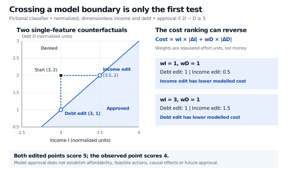
At I=3,D=2, the score is 2(3)−2=4, so the model denies the input. Holding its coefficients and threshold fixed gives two single-feature counterfactuals:
Input
Income
Debt
Score
Model decision
Observed
3
2
4
Denied
Debt edit
3
1
5
Approved
Income edit
3.5
2
5
Approved
The debt edit reduces debt by 1 normalized unit; the income edit increases income by 0.5. Both reach the boundary. They demonstrate model sensitivity, without proving that either edit can actually be achieved.
Fictional normalized classifier approves when twice income minus debt is at least 5. Starting income 3 and debt 2 scores 4. Debt 1 or income 3.5 scores 5. Equal cost weights give costs 1 and 0.5; weighting income by 3 gives costs 1 and 1.5, reversing the ranking.
Original synthetic example. Both edits reach the fixed model’s approval boundary. The preferred edit among these two candidates depends on stipulated action costs; neither path establishes real-world recourse.
Calling one alternative “smallest” requires a distance or cost definition. Suppose the cost assigned to a feature edit is
C(ΔI,ΔD)=wI∣ΔI∣+wD∣ΔD∣.
With both weights equal to 1, the debt edit costs 1 and the income edit costs 0.5. With wI=3,wD=1, their costs become 1 and 1.5. The ranking among these two candidates reverses. These weights are invented effort units, not measured affordability. Rescaling a feature without adjusting its weight also changes what this cost considers close. Wachter and co-authors explicitly discuss the importance of distance and feature scaling in §III.
For background on linear-score geometry, Logistic Regression and Maximum Likelihood develops the decision boundary. The preview is public; the full lesson requires membership.
Restrict the search to available changes
A basic feature-edit formulation is
Δ∈A(x)minC(Δ;x)subject tof(x+Δ)=1.
The set A(x) encodes changes allowed from the observed input. Age must stay fixed in an immediate decision exercise; waiting requires an explicit time horizon, rather than an arbitrary age edit. Discrete variables must retain valid values, and direction and budget restrictions matter. Ustun, Spangher and Liu, §2.1.
For the fictional classifier, suppose the entire permitted action set allows only an income increase between 0 and 0.2 and a debt decrease between 0 and 0.3. The largest reachable score is 2(3.2)−1.7=4.7. No permitted edit reaches 5. This is infeasibility under those stipulated bounds, not a claim about a person's actual options.
Conversely, an optimisation routine merely failing to find a flip does not certify that none exists. A completeness or infeasibility guarantee must be justified for the specified search space. Ustun and co-authors distinguish finding a minimum-cost flip from certifying infeasibility, and discuss customised costs and alternative flipsets in §§2.1 and 3.2–3.4.
A destination is not an action plan
An input may look plausible in a dataset yet be unreachable from this person's situation. A mutable quantity may also be outside their direct control: a recorded score can change without being something the person can simply set.
Causally linked features require particular care. An action that changes earnings could also change other recorded financial quantities. Holding every other column fixed may misrepresent its consequences. A structural causal model can express how an intervention propagates, but its causal assumptions need support. A fitted predictive relationship alone cannot supply them. Karimi, Schölkopf and Valera, §§3–5.
A recourse assessment needs feasible actions, consequences, costs and timing. Karimi and co-authors discuss these practical limits in §5 and Appendix C. The synthetic score assesses neither affordability nor realised repayment. Because our calculation freezes the classifier and input assumptions, its boundary flip cannot promise future approval if the model, threshold, data or decision rules change.
Sources
Wachter, S., Mittelstadt, B. and Russell, C. (2018), Counterfactual Explanations Without Opening the Black Box, §III, pp. 854–855. Fixed-model counterfactual search, distance, scaling and valid inputs. The legal discussion is outside this article's scope.
Ustun, B., Spangher, A. and Liu, Y. (2019), Actionable Recourse in Linear Classification, extended version, §§2.1 and 3.2–3.4. Feasible action sets, cost functions, infeasibility and flipsets.