Local interpretable model-agnostic explanations: Definition & Examples

Local interpretable model-agnostic explanations (LIME) explain an individual model prediction by fitting a simpler model near that input. For a quant inspecting one unusually high risk score, the result offers a readable approximation of the predictor’s behaviour around that case. It does not establish what caused the underlying financial outcome.

The explanation is a surrogate model: its response is fitted to the original model’s predictions, rather than directly to realised returns or defaults. “Model-agnostic” means the explainer can query predictions without inspecting the predictor’s internal structure.

What makes the explanation local?

Ribeiro, Singh and Guestrin (2016) formulate a trade-off between local approximation error and explanation complexity:

\widehat g=\operatorname*{argmin}_{g\in G} \left\{L(f,g,\pi_{x_0})+\Omega(g)\right\}.

Here

f

is the model being explained,

G

is an interpretable model class,

\pi_{x_0}

weights proximity to the chosen input

x_0

, and

\Omega

controls complexity. Perturbed inputs are passed through

f

; the explanation is fitted to those outputs. Its interpretable coordinates can differ from the original features, such as word-presence indicators replacing an embedding.

The paper’s sparse linear procedure includes feature selection. The maintainer’s API documentation also describes selection options and a default Ridge regressor. A small weighted regression without those choices illustrates the mechanism, but does not reproduce the full algorithm.

Three queries, a line, and a visible miss

Consider a synthetic, dimensionless black box

f(x)=x^2

, explained at

x_0=1

. Query three inputs and assign fixed locality weights:

Input $z_i$	Black-box output $f(z_i)$	Weight $w_i$
0	0	0.1
1	1	1
2	4	0.1

Restrict the explanation to

g(x)=a+bx

and choose unpenalised weighted least squares:

\min_{a,b}\sum_{i=1}^3w_i\left[f(z_i)-a-bz_i\right]^2.

This example uses the same scalar coordinate for the model and explanation, keeps both parameters, and performs no feature selection. The weights are stipulated; no random sampling or software defaults enter the calculation.

The weighted means are $\bar z_w=1$ and $\bar f_w=7/6$ . Centring the inputs gives

b=\frac{\sum_iw_i(z_i-1)(f(z_i)-7/6)}{\sum_iw_i(z_i-1)^2} =\frac{0.4}{0.2}=2, \qquad a=\frac76-2=-\frac56.

Consequently,

g(1)=-\frac56+2=\frac76\approx1.166667, \qquad f(1)=1.

The surrogate misses the very prediction being explained by $1/6$ . Minimising a weighted sum of errors does not impose exact interpolation at

x_0

, even though that point has the largest weight.

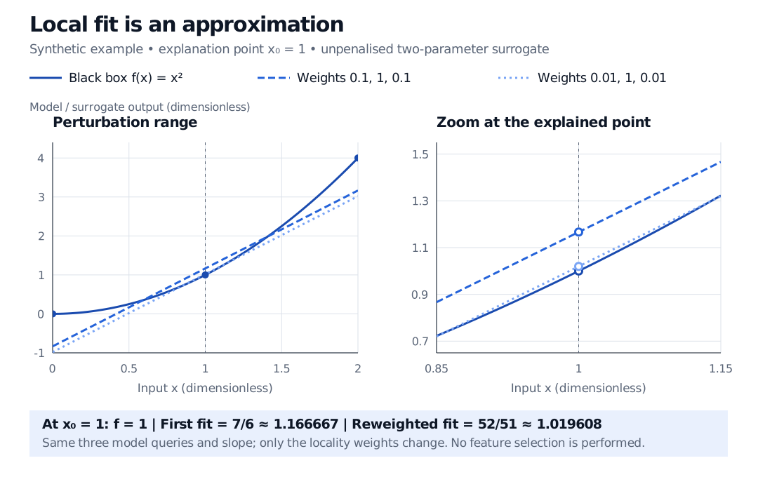
Synthetic dimensionless black box f(x)=x squared is queried at 0, 1 and 2. Weights 0.1, 1 and 0.1 give a line with slope 2 and value 7/6 at x=1, above f(1)=1. Reweighting to 0.01, 1 and 0.01 gives value 52/51, approximately 1.019608. A zoom makes both approximation errors visible.

Synthetic reduced example: the black box and query locations stay fixed. Lower endpoint weights move the unpenalised local line closer to f(1), without making it exact.

Change only the weights to $0.01,1,0.01$ . The slope remains 2, but the intercept becomes $-50/51$ , so $g(1)=52/51\approx1.019608$ . More generally, for symmetric weights $t,1,t$ with $t>0$ ,

g(1)=1+\frac{2t}{1+2t}.

Reducing the distant points’ influence reduces the point error in this particular construction. It is not a guarantee that narrowing a neighbourhood improves every explanation: fewer informative perturbations can leave a fit unstable, and a linear class can miss local curvature or interactions.

For the underlying fitting technique, Beyond Linearity: Splines, Local Regression, and Generalized Additive Models develops distance-weighted local regression. Its preview is public; the full lesson requires membership. LIME differs in fitting the surrogate to a predictor’s queried outputs.

Read the neighbourhood before reading the coefficients

The tabular API exposes sampling, kernel width, distance, discretisation and random-state choices. These choices define the explanation being estimated. Record them, compare repeated samples and sensible neighbourhood definitions, and inspect agreement between the surrogate and the queried model outputs. Local fidelity is an objective to assess, not an automatic guarantee.

In financial data, perturbing related columns independently can generate economically impossible combinations. A price, share count and market capitalisation cannot all vary freely while preserving their accounting relationship. An explanation fitted largely on such off-manifold inputs may describe extrapolation into unsupported states. Valid ranges alone do not preserve joint dependencies.

A coefficient also depends on the chosen coordinates and their scales. A positive local weight for leverage in one risk-score explanation is not evidence that changing leverage would cause a particular realised loss. It describes an approximation under the declared perturbation scheme. One case’s explanation is neither a global feature ranking nor a replacement for model validation.

Sources

Ribeiro, M. T., Singh, S. and Guestrin, C. (2016), “Why Should I Trust You?” Explaining the Predictions of Any Classifier, §§3.1–3.4, equations (1)–(2) and Algorithm 1. Interpretable representations, local loss, complexity and sparse linear explanations; the discussion after Algorithm 1 explains representation and fidelity limits.
LIME maintainers, API reference: LimeBase and LimeTabularExplainer, checked 30 October 2026. Kernel weighting, feature selection, default regression and tabular perturbation controls. The calculation and figure above are original reduced examples, not package output.

What makes the explanation local?

Three queries, a line, and a visible miss

Read the neighbourhood before reading the coefficients

Sources

Related terms

Feature

Feature selection