A concept activation vector turns example-defined concepts into latent directions. TCAV counts positive score sensitivities, with controls needed before interpretation.
Concept activation vector and TCAV
A concept activation vector (CAV) is a direction in a trained neural network's hidden activation space learned to distinguish examples of a human-defined concept from comparison examples. Testing with Concept Activation Vectors (TCAV) measures how model scores respond along that direction across an evaluation set. For a quant analysing financial text, this offers a way to ask whether a classifier's output is sensitive to an example-defined concept such as liquidity-stress language.
That is a diagnostic hypothesis about a model. It does not establish that liquidity stress causes a market outcome.
Turn examples into a direction
Select concept examples and a comparison set, pass both through the frozen network, and fit a linear separator to their activations at a chosen layer. Its normal, oriented toward the concept examples, supplies the CAV. The network itself is not retrained. This is the construction in Kim et al., §§3.2–3.3.
For financial text, concept examples should vary in issuer, date and wording. Otherwise the separator might recognise an issuer name or document template rather than the intended economic idea. Held-out discrimination checks whether the probe generalises; successful discrimination alone does not establish that the target model uses the concept.
Write the layer activation as a=fl(x) and the remaining network's class-k score as hl,k(a). For a unit CAV vC, local directional sensitivity is
The gradient is taken with respect to the chosen layer's activations, holding the network parameters fixed. A positive value means that an infinitesimal step toward the concept direction increases the selected score locally.
A sensitivity of 0.4; a TCAV score of 0.75
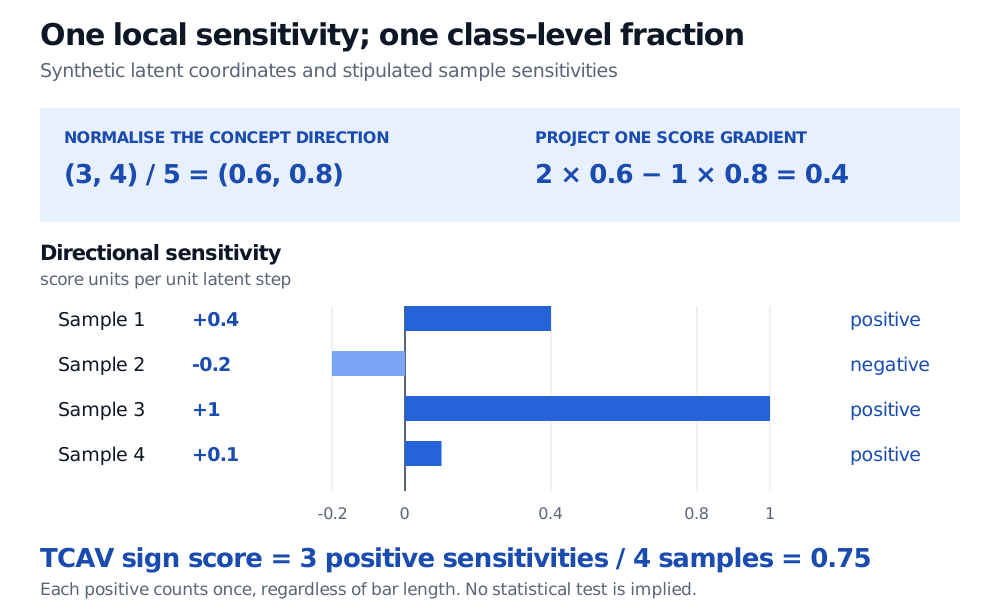
Consider synthetic, dimensionless latent coordinates. Suppose the learned separator normal is (3,4), so normalising it gives vC=(0.6,0.8). At one example, let the score gradient be (2,−1). Then
S=(2)(0.6)+(−1)(0.8)=0.4.
This is a rate of change in score units per unit latent step. It is not a probability or a fraction of explained predictions.
Now stipulate four evaluation examples with sensitivities 0.4,−0.2,1.0,0.1. Only the first uses the preceding gradient; the others are separate stipulated local results. The original TCAV sign score counts strictly positive sensitivities:
Here Xk is the selected class-k evaluation set. The result says that three of four scores locally increase in the concept direction. A zero sensitivity would not count as positive.
Synthetic example: unit concept direction (0.6, 0.8) and score gradient (2, minus 1) give sensitivity 0.4. Four stipulated sensitivities 0.4, minus 0.2, 1 and 0.1 contain three positives, so the TCAV sign score is 0.75.
Original synthetic example. Bar lengths show local directional sensitivities; counting their positive signs gives a different object, the TCAV sign score. The four values are stipulated, not empirical results.
The sign count treats a sensitivity of 0.1 exactly like 1.0. It says nothing about their relative magnitudes. Captum's API documents separate sign-count and magnitude aggregations; specify which statistic is being reported.
Keep the question fixed
A reproducible interpretation names the layer, concept and comparison sets, evaluation population, activation preprocessing and output score. A logit and a multiclass probability are different scores: the probability also depends on competing class logits. Differentiating a training loss answers another question again.
Unit normalisation removes arbitrary CAV length. It does not remove the coordinate system's influence: rescaling individual activation features changes the geometry in which the separator is fitted. If preprocessing activations, express the direction and score gradient in compatible coordinates. Comparisons across layers or preprocessing choices need renewed checks.
A latent step need not correspond to any feasible edit of the original document or market state. Consequently, even a large sensitivity or a high sign score provides no causal effect, predicted return or percentage of the prediction “explained.”
Controls before a conclusion
Repeat the CAV fit with different comparison samples and check stability. Include negative controls, such as random-concept-versus-random-concept comparisons, to see whether apparently strong scores arise without a coherent concept. The Captum tutorial's statistical-testing section illustrates repeated comparison sets and random controls.
Specify the null hypothesis and experimental unit before applying a hypothesis test. Repeated probe fits sharing documents are not automatically independent evidence about new financial periods. Account for multiple testing when screening many concepts or layers. The four-example illustration above contains no significance result; its 0.75 alone supports no claim of a meaningful concept relationship.
For the derivative machinery, Backpropagation as the Chain Rule has a public preview; the full lesson requires membership. TCAV uses that machinery with the selected output score and hidden activations as the derivative's endpoints.