Chen–Roll–Ross factor model: Definition & Examples

The Chen–Roll–Ross factor model is a macroeconomic specification of stock returns using industrial production, inflation and bond-market variables. It gives a quant economically named sources of systematic risk, so a portfolio's sensitivity to the economy can be studied beyond a single market beta. It is associated with Chen, Roll and Ross's 1986 paper, Economic Forces and the Stock Market.

The distinction from arbitrage pricing theory matters: APT supplies a pricing argument under its assumptions; it does not select this particular list of factors.

What the five inputs mean

The familiar specification uses these variables. Expectations below are conditional on information available at the indicated month-end.

Symbol	Original construction
$MP_t$	Monthly log growth in US industrial production: $\log(IP_t/IP_{t-1})$ .
$DEI_t$	Change in expected inflation: $\mathbb{E}[I_{t+1}\mid t]-\mathbb{E}[I_t\mid t-1]$ .
$UI_t$	Realised inflation less its prior expectation: $I_t-\mathbb{E}[I_t\mid t-1]$ .
$UPR_t$	Return on a Baa-and-under corporate-bond portfolio minus long-term government-bond return.
$UTS_t$	Long-term government-bond return minus the one-month Treasury-bill rate known at $t-1$ for month $t$ .

The bond variables are return differences, not simply corporate-minus-government or long-minus-short yield levels. Nor are all five series mechanically forecast residuals: the authors explicitly note that

UPR

is not formally an innovation, and treating

DEI

as one requires an assumption about expected inflation. Their statistical alignment also leads monthly production by one month. These details matter when reproducing the original study. Original constructions, §III and Table 1.

A macro factor is therefore a measured series with a timing rule, not just a label such as “inflation”. Replacing the expectation model, bond portfolio or data vintage creates a different empirical implementation.

Exposures explain movements; prices of risk explain expected returns

Write a centred-input version of the return equation as

R_{i,t}=a_i+\sum_{k=1}^{5}b_{i,k}x_{k,t}+\varepsilon_{i,t}.

Here $x_{k,t}$ is a declared centred factor input, $b_{i,k}$ is its factor exposure, and $\varepsilon_{i,t}$ is the asset-specific residual. A time-series regression estimates the loadings from repeated observations of the asset and the factors. Centring changes the intercept; it does not by itself turn an input into an unpredictable economic shock.

A separate cross-sectional pricing question is whether assets with different loadings have different expected returns:

\mathbb{E}[R_i]=\lambda_0+\sum_{k=1}^{5}b_{i,k}\lambda_k.

The $\lambda_k$ are prices of factor risk, not the realised $x_{k,t}$ and not the loadings $b_{i,k}$ . Estimating exposures is only the first step toward a Fama–MacBeth regression pricing test. A large loading or a good time-series fit alone does not establish a nonzero factor premium.

A fictional attribution calculation

Suppose a portfolio has the following sensitivities. Every input is a fictional centred value in percentage points; each loading converts one input percentage point into return percentage points. These are neither the original paper's estimates nor its factor normalisations.

Input	Centred value (pp)	Loading	Return contribution (pp)
Production	0.50	1.20	+0.60
Change in expected inflation	0.20	−0.50	−0.10
Unexpected inflation	−0.10	0.80	−0.08
Risk-premium spread	0.30	0.60	+0.18
Term structure	0.40	−0.30	−0.12

Multiplying each input by its loading gives a net factor contribution of

0.60-0.10-0.08+0.18-0.12=0.48\text{ percentage points}.

Fictional contributions: production plus 0.60, expected inflation minus 0.10, unexpected inflation minus 0.08, risk premium plus 0.18 and term structure minus 0.12 percentage points; net plus 0.48.

Positive production and risk-premium contributions outweigh the three negative contributions. The net excludes the intercept and residual.

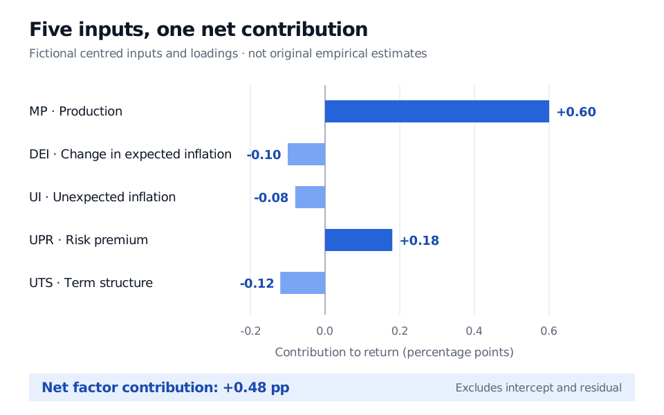
This is factor attribution under an assumed linear model. It is not the portfolio's complete return, an expected risk premium or a causal estimate. For example, the negative unexpected-inflation contribution follows from a positive loading multiplied by a negative input; it does not establish a universal rule about how stocks respond to inflation.

Loadings must accompany their units. Expressing the same inputs in smaller units requires inversely rescaling the loadings to preserve the fitted return. There is no fixed universal coefficient vector to copy into a trading system.

Using the specification carefully

For risk monitoring, document the factor definitions, observation frequency, release calendar, expectation model and estimation window before interpreting exposures. A historically aligned production series can be useful in a research test while being unavailable for a contemporaneous trading decision. Check what information actually existed at the decision time.

The model offers an interpretable research specification, not a guarantee that these variables price every asset universe or remain significant in a new sample. A new application needs its own estimation, uncertainty assessment and pricing tests.

For a foundation in interpreting slopes, residuals and the limits of fitted relationships, read Basic Statistics and Regression. The full primer lesson requires a free account.

Sources

Chen, N.-F., Roll, R. and Ross, S. A. (1986). Economic Forces and the Stock Market, The Journal of Business, 59(3), 383–403. §III and Table 1 define the inputs; §IV.A distinguishes estimated exposures from the subsequent pricing test. Publisher DOI.

What the five inputs mean

Exposures explain movements; prices of risk explain expected returns

A fictional attribution calculation

Using the specification carefully

Sources

Related terms

Systematic risk