Cartea–Jaimungal market-making model: Definition & Examples

The Cartea–Jaimungal market-making model is a stochastic-control framework for choosing bid and ask quotes using inventory, execution conditions and predictions of short-term price moves. Its practical consequence is that a quote can change because the maker's position changed, because the expected value of holding the asset changed, or because the flow likely to fill the quote became more dangerous.

The name covers related specifications. Here the research reference is Cartea, Jaimungal and Ricci's 2014 mutually exciting order-flow model, Buy Low, Sell High, with its 2018 author exposition also used below. Ricci is a coauthor of this version. It extends market making beyond a static choice of spread around a fair price. The original paper specifies the model in §§2–5.

What the maker controls

The controls are continuously revised quote distances: ask $S_t+\delta_t^+$ and bid $S_t-\delta_t^-$ . Orders have fixed unit size. Cash is $X_t$ , inventory is $q_t$ , and $S_t$ is the midpoint. The objective in §5.1 is

\sup_{\delta^+,\delta^-}\mathbb{E}\left[X_T+q_TS_T-\phi\int_t^T q_u^2\,du\mid\mathcal{F}_t\right].

It maximises expected marked terminal wealth while charging for carrying inventory throughout the path. With inventory measured in shares, prices in USD/share and time in seconds,

\phi

has units USD/(share²·second). This is a preference penalty, not a cash fee. The specified terminal value marks remaining inventory at the midpoint; it neither forces

q_T=0

nor includes a separate terminal liquidation penalty. Cartea, Jaimungal and Ricci (2014), §5.1.

A fill changes more than inventory

In this version, the midpoint has a short-term drift component

\alpha_t

. Influential market orders can change that drift, future buy/sell arrival rates and the book-shape state governing fills. These effects mean-revert. A market order can therefore change the maker's continuation value even when its own quote does not fill. The dynamic programme includes both branches. The 2018 author exposition, §§2–5.

A positive drift forecast encourages retaining or acquiring inventory; inventory risk can pull the other way. Avoiding adverse selection requires valuing a fill conditional on the event and resulting state, rather than using unconditional price drift. Here $\alpha_t$ is price change per unit time, not an expected total gain per share over the remaining horizon.

The model factors a fill rate into a market-order arrival rate and the conditional probability that the order reaches the posted depth. An arrival is not automatically a fill. It is a reduced description of order flow, not an explicit queue-position simulator. The original paper, §3 and §5.

This differs from the original Avellaneda–Stoikov model, which uses exponential utility of terminal wealth, a driftless Brownian midpoint and depth-dependent Poisson executions. Inventory skew is common to both; their objectives and information dynamics differ. Avellaneda and Stoikov (2008), §§2–3.

Read the quote calculation before calling it a policy

The following fictional reduced calculation isolates the local quote decision. It does not solve the mutually exciting model above.

Assume one-share fills, a frozen midpoint of USD 100/share, no fees, and nonnegative continuous quote depths. Each side's fill intensity is

\Lambda(\delta)=\lambda_0e^{-k\delta},\qquad k=20\text{ per USD/share}.

Here $\lambda_0>0$ is a baseline rate per second. Equivalently, conditional on a corresponding market-order arrival, the stipulated fill probability is $e^{-k\delta}$ . For this calculation, a fill changes cash and inventory only: no signal, arrival-rate or book-shape jump is coupled to that event. In a short interval $dt$ , the fill probability is $\Lambda(\delta)dt+o(dt)$ , not $\Lambda(\delta)$ itself.

Supply an inventory continuation adjustment $H(q)$ , measured in total USD, with $q$ the numerical number of shares. At the current state, selling one share changes marked wealth plus this adjustment by

\delta^+ + H(q-1)-H(q).

The ask's local objective is therefore

\lambda_0e^{-k\delta^+}\bigl[\delta^+ + H(q-1)-H(q)\bigr].

The bid uses $H(q+1)-H(q)$ . Differentiating each objective gives the constrained optima

\begin{aligned} \delta^{+*}&=\max\{0,\ 1/k+H(q)-H(q-1)\},\\ \delta^{-*}&=\max\{0,\ 1/k+H(q)-H(q+1)\}. \end{aligned}

For an interior optimum, the derivative changes from positive to negative at this point. The baseline intensity scales the objective without changing its maximiser when the continuation values are held fixed. In a solved dynamic model, those values themselves depend on execution opportunities.

Set $q=5$ and stipulate $H(q)=-0.001q^2$ USD. Then $H(5)=-0.025$ , $H(4)=-0.016$ and $H(6)=-0.036$ dollars. Since $1/k=0.05$ USD/share, the depths are

\delta^{+*}=0.05-0.009=0.041,\qquad \delta^{-*}=0.05+0.011=0.061.

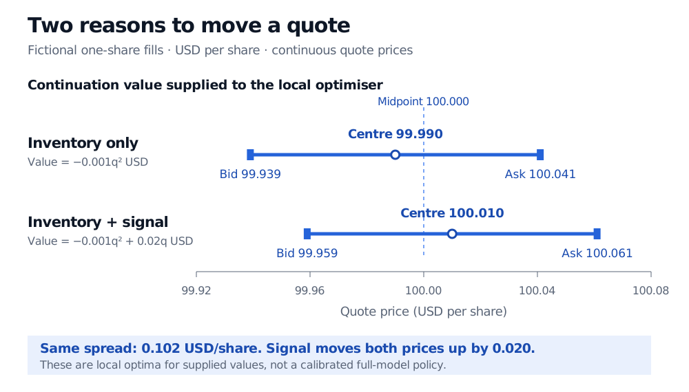
The long maker sells more readily and buys less readily: bid 99.939 / ask 100.041, centred at 99.990.

Now supply

H(q)=-0.001q^2+0.02q

USD instead. The linear term values each additional share at another USD 0.02. It raises ask depth by 0.02 and lowers bid depth by 0.02:

Supplied continuation value	Bid depth	Ask depth	Bid / ask	Quote centre
Inventory term only	0.061	0.041	99.939 / 100.041	99.990
Inventory plus signal value	0.041	0.061	99.959 / 100.061	100.010

All depths and quote prices are USD/share. The signal value outweighs the downward inventory skew, so the centre moves above the midpoint. Both full spreads equal 0.102 USD/share.

Fictional local quote optima at midpoint USD 100 per share. Inventory alone gives bid 99.939, ask 100.041 and centre 99.990. Adding a stipulated signal value gives bid 99.959, ask 100.061 and centre 100.010. Both full spreads are 0.102.

Original reduced-control illustration with one-share fills and supplied continuation values. Signal value shifts both quotes up by USD 0.020 per share; the full spread stays USD 0.102 per share.

The 0.02 is a continuation-value increment, not an instantaneous drift. Neither supplied

H

has been obtained by solving the full model's Hamilton–Jacobi–Bellman equation. The paper's exponential-fill feedback formula also contains event-conditioned state updates; dropping those updates is an additional simplifying assumption. Its derivation is in Appendix C.1 of the original paper.

From a model to executable quotes

The example allows fractional-cent prices and immediate revision. An actual venue imposes ticks, order priority and cancellation delays; admissible quotes must respect those constraints. Fees and liquidation costs change the objective. A fill model estimated for one queue position or market regime need not remain valid elsewhere. A numerical optimum under a misspecified fill law can simply be a precise answer to the wrong execution problem.

The supporting lesson Order Flow and Adverse Selection develops conditional fill losses and the limits of interpreting persistent flow as informed trading. Its preview is public; the full lesson requires membership.

Sources

Cartea, Á., Jaimungal, S. and Ricci, J. (2014), Buy Low, Sell High: A High Frequency Trading Perspective, SIAM Journal on Financial Mathematics 5(1), 415–444. Linked author preprint dated 15 April 2014: §§2–5 and Appendix C.1, especially the fill-rate assumptions, objective (6) and feedback formula (C.1a).
Cartea, Á., Jaimungal, S. and Ricci, J. (2018), Algorithmic Trading, Stochastic Control, and Mutually-Exciting Processes, SIAM Review 60(3), 673–703. Author version: §§2–5, including the state transitions in the HJB. This is a later exposition of the framework, not the date of the original paper.
Avellaneda, M. and Stoikov, S. (2008), High-frequency trading in a limit order book, Quantitative Finance 8(3), 217–224, §§2–3. Used to distinguish the original utility-based inventory model.

What the maker controls

A fill changes more than inventory

Read the quote calculation before calling it a policy

From a model to executable quotes

Sources

Related terms

Market making

Order flow