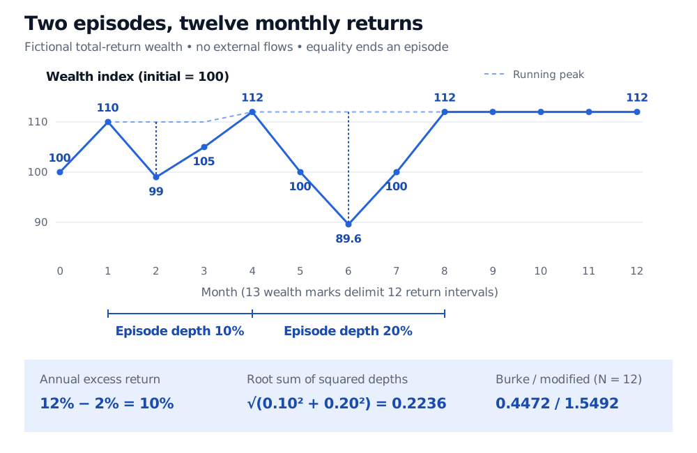
The Burke ratio compares excess return with squared drawdown losses. A monthly example separates full underwater episodes, negative-return runs and modified normalisation.
Burke ratio
The Burke ratio divides portfolio return above a risk-free comparator by the square root of the sum of squared drawdowns. It measures reward relative to several historical loss events, with deeper events contributing disproportionately. In a strategy comparison, this can reveal repeated losses that a denominator based only on maximum drawdown would overlook. But the result is meaningful only after defining what counts as one drawdown.
The event definition is part of the ratio
Write the ratio as
B=∑j=1KDj2rP−rf,
where Dj is a positive fractional loss magnitude for event j, and K is the number of included events. Here rP is the annual geometric portfolio return and rf an annual effective risk-free comparator in the same currency. Other numerator conventions exist; an annual arithmetic mean is not interchangeable with geometric growth.
This article's worked convention is full peak-to-recovery episodes. Starting from positive, cash-flow-adjusted total-return wealth W0,…,WN, define the running peak and current loss magnitude:
Ht=0≤s≤tmaxWs,dt=1−HtWt.
An episode starts when wealth falls below its running peak and ends when it reaches or exceeds that peak. Its depth Dj is the largest dt inside the episode. A rebound that remains below the peak does not create a new episode. We include every episode, without a minimum-loss filter or restriction to the largest few. If the window ends underwater, include that open episode's observed depth and identify it as unfinished; its eventual depth and recovery time remain unknown.
This is a declared convention, not a uniquely universal historical definition. In Carl Bacon's discussion, printed page 10 describes individual drawdowns as continuous negative-return periods, distinguishing them from the maximum peak-to-trough loss. Page 12 uses the root sum of squared individual drawdowns for Burke and allows restricting the count to the largest events. A report following that negative-return-run convention can disagree with the full-episode convention above.
For example, consider the fictional wealth path 100 → 90 → 95 → 85 → 100. It contains one full underwater episode, with depth 15%. It contains two negative-return runs: 100 to 90 loses 10%, and 95 to 85 loses 10/95≈10.5263%. The rally to 95 ends a negative run but does not recover the high of 100. These event lists must not be silently substituted for each other.
Twelve monthly returns, two episodes
Suppose a fictional portfolio has the following month-end total-return wealth, including its initial mark. There are no external flows; income is reinvested and the wealth index is net of the assumed costs.
Month
Wealth index
Episode status
0
100
Initial peak
1
110
New peak
2
99
First episode trough
3
105
Still below 110
4
112
Recovery and new peak
5
100
Second episode underway
6
89.6
Second episode trough
7
100
Still below 112
8
112
Recovery to equal peak
9–12
112 each month
At the peak
The two episode depths are
D1=1−11099=0.10,D2=1−11289.6=0.20.
Terminal wealth is 12% above initial wealth over exactly one year. With a stipulated annual effective risk-free return of 2%, annual excess return is 0.12−0.02=0.10. Therefore
B=0.102+0.2020.10=0.22360680.10≈0.4472136.
The 20% episode contributes four times as much squared loss as the 10% episode. Both remain in the denominator after recovery. The ratio is neither a probability nor a statement that future losses are bounded by these observations.
Fictional monthly wealth starts at 100 and ends at 112. An episode from month 1 to month 4 has depth 10 percent; an episode from month 4 to month 8 has depth 20 percent. Annual excess return is 10 percent. Burke ratio is 0.4472 and modified Burke with 12 return observations is 1.5492.
Original fictional monthly example. The 13 wealth marks delimit 12 returns; drawdown depths use full peak-to-recovery episodes, with equality counted as recovery.
“Modified” changes the normalisation
The PerformanceAnalytics documentation gives a modified Burke formula that divides the sum of squared event losses by the number of observations in the entire return series:
Bmodified=N1∑j=1KDj2rP−rf=NB.
Applying that normalisation to our declared episode list, N=12 monthly return observations, not two episodes and not 13 wealth marks. Thus
Bmodified=(0.102+0.202)/120.10≈1.5491933.
This square-root multiplier is a sample-size normalisation, not a general annualisation rule. For equal N, modified and unmodified Burke give the same ordering. Different observation counts introduce different multipliers, so changing sampling frequency or window length can change comparisons.
Normalising an episode sum does not turn it into the Ulcer Index. The Ulcer Index squares the drawdown at every sampled date and averages across the declared full set of dates, including dates at the peak. As Peter Martin's calculation shows, repeated underwater dates enter repeatedly. The Martin ratio uses that denominator. Here an episode contributes its deepest loss once; extra time at the same trough does not add another event.
What a reproducible comparison must state
An implementation's name is insufficient. The maintainer's BurkeRatio source, inspected on 31 October 2026, identifies negative-return runs and compounds their losses with percentage conversions, while its portfolio-return calculation uses decimal returns. It is therefore unsafe to assume that feeding decimal returns into that implementation reproduces the full-episode calculation here. Verify event extraction and units against a transparent wealth path before comparing outputs.
For any Burke report, specify the measurement dates, valuation frequency, event definition, open-episode policy, event filters, numerator and normalisation. Keep return and drawdown units consistent: using 10 and 20 percentage points instead of 0.10 and 0.20 gives the same ratio only if the excess-return numerator is also multiplied by 100. Annualising the numerator does not supply a square-root-time scaling law for the drawdown denominator.
The starting high-water mark matters too. Resetting it at the window boundary can hide a loss from an earlier peak. Coarse or stale valuations can miss intraperiod losses. A longer record can add events to the unnormalised sum even when the annual return is similar. A zero event-loss denominator makes the ratio undefined. With negative excess return, a larger denominator moves the ratio towards zero, so the usual “higher is better” interpretation needs particular care.
For the broader evaluation process, Backtest Evaluation develops flow-adjusted wealth, drawdown recovery and reporting of research uncertainty. The public page is a preview; the full lesson requires membership.