Blume and Vasicek beta adjustment: Definition & Examples

Blume and Vasicek beta adjustment are methods for pulling an estimated market beta toward a reference value before using it in risk analysis. A common Blume-style rule applies the same pull to every stock. Vasicek-style adjustment makes the pull depend on how uncertain each estimate is relative to the prior dispersion of betas. The choice can materially change an exposure estimate used in a hedge or a portfolio risk model.

A raw beta is a fitted slope, not an observed constant of nature. Keep the benchmark, return frequency, currency, estimation window and return convention attached to it. Shrinking a poorly specified regression does not repair its specification.

A common rule and its historical interpretation

A widely used Blume-style convention is

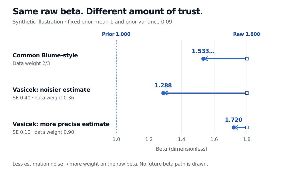
\hat\beta_{\mathrm{B}}=\frac23\hat\beta+\frac13(1).

It retains two-thirds of the raw estimate's distance from one. A synthetic raw beta of $1.8$ becomes

\hat\beta_{\mathrm{B}}=\frac23(1.8)+\frac13=\frac{23}{15}\approx1.5333.

Blume's empirical approach fitted a linear relationship between beta estimates from successive periods. The intercept and slope were estimated; the two-thirds rule is a common simplified convention, not universal coefficients from Blume's original research. Welch, Section II.B, separates the fitted historical correction from that convention. Damodaran's Post-Regression Beta Adjustments in Practice, PDF p. 10, illustrates the closely related rounded weights

0.67

and

0.33

A constant rule treats a precisely estimated beta and an imprecisely estimated beta alike. That is the useful contrast with Vasicek adjustment.

Vasicek: let precision determine the pull

To expose the mechanism, stipulate a Gaussian measurement model for one stock:

\hat\beta=\beta+\varepsilon,\qquad \varepsilon\sim\mathcal N(0,s^2),\qquad \beta\sim\mathcal N(\mu,\tau^2),

with the estimation error independent of the latent beta and positive, known variances. Here

s^2

is the sampling variance of the raw beta estimate, while

\tau^2

describes prior dispersion of the latent beta. Neither is the variance of the stock's returns. Treating an estimated regression standard error as known is a plug-in approximation to this illustration.

Multiplying the normal likelihood and prior and completing the square gives

\begin{aligned} \mathbb E[\beta\mid\hat\beta] &=w\hat\beta+(1-w)\mu, & w&=\frac{\tau^2}{\tau^2+s^2},\\ \text{Var}(\beta\mid\hat\beta) &=\left(\frac1{\tau^2}+\frac1{s^2}\right)^{-1} =\frac{\tau^2s^2}{\tau^2+s^2}. \end{aligned}

The weight $w$ is the data's share of total precision: $(1/s^2)/(1/s^2+1/\tau^2)$ . A larger standard error means less weight on the raw estimate. Greater prior heterogeneity means more weight on it. This is a shrinkage estimator built from Bayesian inference; Welch's Section II.B gives a cross-sectional implementation of the Vasicek estimator.

For the same raw beta $1.8$ , use prior mean $\mu=1$ , prior variance $\tau^2=0.09$ and sampling variance $s^2=0.16$ , corresponding to standard error $0.4$ . Then

w=\frac{0.09}{0.09+0.16}=0.36, \qquad \mathbb E[\beta\mid\hat\beta]=0.36(1.8)+0.64(1)=1.288.

The conditional posterior variance is $0.0576$ , with standard deviation $0.24$ . These quantify uncertainty about beta under the stipulated model; they are not a forecast of return volatility.

Now change only the sampling variance to $0.01$ (standard error $0.1$ ). The data weight rises to $0.9$ and the adjusted beta becomes $0.9(1.8)+0.1(1)=1.72$ . The more precise estimate stays closer to its raw value.

Synthetic raw beta 1.8 and prior mean 1: the common Blume-style adjustment gives 1.5333, Vasicek with standard error 0.4 gives 1.288, and Vasicek with standard error 0.1 gives 1.72.

Original synthetic comparison. The Vasicek cases share prior mean 1 and prior variance 0.09. Only estimation precision changes; the arrows describe adjusted estimates, not future beta paths.

Choosing a prior is part of the model

The prior centre need not be one. An industry or another economically coherent peer group can imply a different $\mu$ . One is the benchmark's beta against itself; it is not automatically the equally weighted mean beta of an arbitrary stock sample.

Estimating $\mu$ and $\tau^2$ from other securities introduces an empirical Bayes step. Be explicit about whether an implementation uses raw cross-sectional dispersion as a practical proxy or estimates latent heterogeneity after accounting for measurement noise. Under the simple independent measurement model with a common sampling variance,

\text{Var}(\hat\beta)=\tau^2+s^2.

Thus the spread of noisy estimated betas is not, in general, the spread of their underlying true betas. Unequal sampling errors and correlated errors require more care. A posterior calculation that plugs in estimated prior parameters also omits uncertainty about those parameters.

For the algebra behind the update, read The Normal-Normal pair, Theorem 3 in Conjugate Prior Families. The full lesson requires membership, with a public preview; it derives the precision sum and posterior mean used here.

Shrinkage does not establish future mean reversion

The Gaussian example can shrink a noisy estimate even when the latent beta is constant. Actual changes in business mix, leverage or market conditions are a separate source of changing exposure. Forecasting a future beta needs assumptions about that evolution and a stated forecast horizon. A smaller adjusted estimate does not establish that the stock's future beta will move toward one, or that every stock benefits from the same adjustment.

Report the raw estimate, its uncertainty, the target and the adjustment rule together. Assess forecast performance against the intended future exposure measure using information available at the estimation date. A shrinkage formula alone supplies no universal improvement guarantee for every stock or regime.

Practice

A synthetic stock has raw beta $0.4$ and sampling variance $0.12$ . An independently specified Gaussian prior has mean $1.2$ and variance $0.04$ . What is its posterior mean under the same measurement model, and does the adjustment lower its beta?

Answer. The data weight is

0.04/(0.04+0.12)=0.25

, giving

0.25(0.4)+0.75(1.2)=1.0

. The adjustment raises beta toward the prior centre

1.2

. Shrinkage reduces distance from the target; it does not necessarily reduce the number, and its target need not be one.

Sources

Ivo Welch, Simply Better Market Betas, author manuscript dated 13 June 2021, Section I, pp. 3–4, and Section II.B, pp. 7–8: estimation targets, the implemented Vasicek weights, the fixed-beta derivation versus changing exposures, and Blume's fitted correction versus the simplified two-thirds convention.
Aswath Damodaran, Estimating Risk Parameters, NYU Stern, PDF pp. 10–11 and 14–16: common post-regression adjustment, estimation noise and changes in the firm's exposure. The numerical cases and figure here are original stipulated examples.