A bipartite matching selects pairs between two disjoint sets so that each item appears in at most one pair. Each edge in the graph marks an eligible pair. In trade reconciliation, the two sets might be internal fills and broker records. A maximum-cardinality matching produces as many reconciled pairs as the one-to-one rule permits. That rule fits feeds with one record per fill. Split or aggregated records require a model that allows multiple links per record.
How to free a record that's already paired
Consider a fictional batch. Fill A is eligible for records x and y, fill B only for x, and fill C for y and z. Suppose a greedy algorithm has selected A–x and C–y. B and z are the only free endpoints and there is no edge between them. The two pairs form a maximal matching, meaning no single edge can be added while keeping the existing pairs.
Start at B and follow its only eligible edge to x. Trace x's current pair back to A, then try A's unused edge to y. Record y is paired with C, whose unused edge leads to the free record z. The route B–x–A–y–C–z is an augmenting path. Its edges alternate between unused and selected, and both endpoints are free.
Flip the path in one update. Remove A–x and C–y, and add B–x, A–y and C–z. Each interior vertex swaps one partner for another, while the two endpoints gain partners. The count rises from two to three pairs, the largest possible with three fills and three broker records. Every vertex is now matched, so this is also a perfect matching.
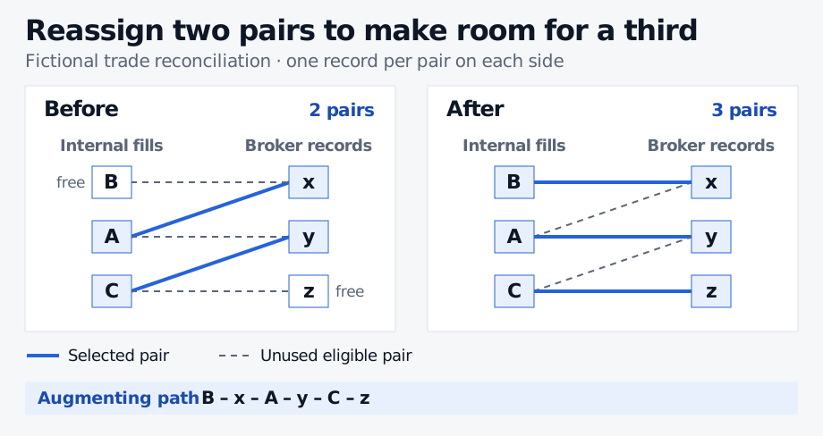
The same eligibility graph before and after the flip. Each interior vertex changes partners, and the two free endpoints gain partners.
In general, a matching is maximum exactly when it has no augmenting path. To look for one, search from free vertices on the left. Follow unused edges left to right and selected edges right to left, stopping if you reach a free vertex on the right. Flip the path and repeat. Cornell CS 6820, Matchings, §§1.2–1.3
The same search can be expressed as a maximum-flow problem. Add a source that feeds the left vertices and a sink that receives flow from the right vertices. Direct the eligibility edges left to right and give every edge capacity one. An integral maximum flow exists. Its middle edges with one unit of flow are the matched pairs. Fractional feasible flows, including some maximum flows, can split one unit across multiple edges. The SelfMadeQuant lesson on maximum flow diagrams the network construction. The preview is public and the full lesson requires membership. Chuzhoy and Khanna, §1.1
When eligible pairs have costs
If every item must be paired and a perfect matching exists, the classical linear assignment problem chooses the perfect matching with the lowest total cost . In reconciliation, could be the absolute timestamp difference in seconds for an eligible pair. The balanced assignment has a linear programming formulation, and the Hungarian method is one way to solve it. Michel X. Goemans, §2
When some records may remain unmatched and coverage comes first, maximise the number of pairs, then minimise the cost among matchings of that size. Minimising total cost alone with positive costs and optional matches would choose the empty matching.